Before discussing the canonical formulation of Einstein’s TGR and the relation it bears to string-dynamics and the critical relation between the total string-theory action and the Nieh–Yan-Barbero-Immirzi action, note that the Hilbert action is a functional of the metric tensor, given by:
![\[{S_D} = {\int {\left( {^{\_\left( 4 \right)}g} \right)} ^{1/2}}{\,^{\left( 4 \right)}}R{d^4}x\]](https://www.georgeshiber.com/wp-content/ql-cache/quicklatex.com-3d08ac009e8cc514757118b38dddd735_l3.png "Rendered by QuickLaTeX.com")
also note a crucial relation to the D-p-brane partition function for closed strings, which is:
![\[P_{{\rm{int}}}^{Dp} \equiv \not Z = \sum\limits_{\gamma = 0}^\infty {\underbrace {\int {{{\not D}^{SuSy}}\gamma {{\not D'}^{SuSy}}X{e^{S_{cld}^s}}} }_{{\rm{Topologies}}}} \]](https://www.georgeshiber.com/wp-content/ql-cache/quicklatex.com-6b94ce686f3d93b2aa0ad1ef5d9550c3_l3.png "Rendered by QuickLaTeX.com")
where  is the supersymmetry group covariant derivative. Since the closed string action satisfies the variational equation:
![\[\begin{array}{c}\delta S_{cld}^s = - \frac{1}{{2\pi \alpha '}}\int_{\partial E_S^5} {{d^2}} \sigma d\,\Omega {\left( {{\phi _{INST}}} \right)^2}{\varepsilon ^{\alpha \beta }}{{\not \partial }_\alpha }{X^\mu }{{\not \partial }_\mu }{\lambda _\nu }\\ = - \frac{1}{{2\pi \alpha '}}\int_{\partial E_S^5} {{d^2}} d\,\Omega {\left( {{\phi _{INST}}} \right)^{ - 1/2}}\sigma \,{{\not \partial }_\mu }X\nu {\left( {{\varepsilon ^{\alpha \beta }}{{\not \partial }_\beta }{X^{^\nu }}{\lambda _\mu }} \right)^{{e^{ - H_3^b}}}}\end{array}\]](https://www.georgeshiber.com/wp-content/ql-cache/quicklatex.com-5bb7f2eeea6ee05059227d9661afdb33_l3.png "Rendered by QuickLaTeX.com")
it follows that no topology in the sum is degenerate, and hence the closed string has a solvable action in 4-D curved space-time described by  that needs no renormalization, where the closed string action coupled to the instanton field is:
![\[\begin{array}{*{20}{c}}{S_{cld}^s = - \frac{1}{{4\pi \alpha '}}\int_{\partial E_{{S_D}}^5} {{d^2}} \sigma d{\mkern 1mu} \Omega {\mkern 1mu} {{\left( {{\phi _{INST}}} \right)}^2}\sigma \sqrt { - \gamma } \left( {\phi \left( {\bar X} \right)} \right.{R_{icci}} + {\gamma ^{\alpha \beta }}{\partial _\alpha }{X^\mu }{g_{\mu \nu }}\left( {\bar X} \right)}\\{ + \frac{1}{{\sqrt { - \gamma } }}{\varepsilon ^{ - H_3^b}}{\partial _\alpha }{X^\mu }{\varepsilon ^{\alpha \beta }}{\partial _\beta }{X^\nu }{b_{\mu \nu }}{{\left( {\bar X} \right)}^2}}\end{array}\]](https://www.georgeshiber.com/wp-content/ql-cache/quicklatex.com-e8f53fedd6e19604d15247770b80db2c_l3.png "Rendered by QuickLaTeX.com")
Recall that in the canonical formalism for Einstein’s TGR as developed by Dirac and Arnowitt, Deser and Misner (ADM), standardly but wrongly identified with loop quantum gravity, the Hilbert action is a functional of the metric tensor, given by:
![\[{g_{\mu \nu }}(x),\quad x \in {\mathbb{R}^4}\]](https://www.georgeshiber.com/wp-content/ql-cache/quicklatex.com-bd652d06c837e0ca5a2718d52f07480b_l3.png "Rendered by QuickLaTeX.com")
A central property of the Hilbert action is that one can add a divergence term to the integrand in:
by substituting the Dirac-ADM Lagrangian density:
![\[L_D^{adm} = {\left( {^{ - (4)}g} \right)^{1/2}}{\,^{(4)}}R + \frac{{\partial {{\tilde V}^\alpha }}}{{\partial {x^\alpha }}}\]](https://www.georgeshiber.com/wp-content/ql-cache/quicklatex.com-255dba0be7500ee5f9233a4f91a645f6_l3.png "Rendered by QuickLaTeX.com")
thus eliminating all occurrences of second derivatives of  and no first-time derivatives of
  . The important point being is that have vanishing conjugate momenta and occur in the theory as arbitrary functions, thus the remaining degrees of freedom are those represented by the spatial metric components
  and their conjugates
  , and both fields are related as:
![\[\begin{array}{l}{{\rm H}_ \bot } = {g^{ - 1/2}}\left( {{\pi _{ij}}{\pi ^{ij}} - \frac{1}{2}{{\left( {\pi _j^i} \right)}^2}} \right) - \\{g^{1/2}}/R \approx 0\end{array}\]](https://www.georgeshiber.com/wp-content/ql-cache/quicklatex.com-fcfb145b6c0a0e46daa4897d11ed4c26_l3.png "Rendered by QuickLaTeX.com")
and
![\[{{\rm H}_i} = - 2{\pi _i}^j\left| {_j} \right. \approx 0\]](https://www.georgeshiber.com/wp-content/ql-cache/quicklatex.com-403fd694c8ee3639f1aee5ef75027e5f_l3.png "Rendered by QuickLaTeX.com")
the geometric upshot is that  generate arbitrary reparametrizations of the spacelike hypersurface on which the state is defined and
  generate deformations that change the location of the hypersurface in the ambient spacetime
generate arbitrary reparametrizations of the spacelike hypersurface on which the state is defined and generate deformations that change the location of the hypersurface in the ambient spacetimeHence, the hypersurfaces are embedded in a common spacetime, mathematically expressed by the following relations:
![\[\begin{array}{l}\left[ {{{\rm H}_ \bot }\left( x \right),{{\rm H}_ \bot }\left( {x'} \right)} \right] = \left( {{g^{rs}}\left( x \right){{\rm H}_s}\left( x \right)} \right.\\ + {g^{rs}}\left( {x'} \right)\left. {{{\rm H}_s}\left( {x'} \right)} \right){\delta _{,r}}\left( {x,x'} \right)\end{array}\]](https://www.georgeshiber.com/wp-content/ql-cache/quicklatex.com-031fdd53554aa0496110b4ee3374a666_l3.png "Rendered by QuickLaTeX.com")
![\[\left[ {{{\rm H}_r}\left( x \right),{{\rm H}_ \bot }\left( {x'} \right)} \right] = {{\rm H}_ \bot }\left( x \right){\delta _{,r}}\left( {x,x'} \right)\]](https://www.georgeshiber.com/wp-content/ql-cache/quicklatex.com-c521f9263eb5e8029c220532fe7b0050_l3.png "Rendered by QuickLaTeX.com")
and
![\[\begin{array}{l}\left[ {{{\rm H}_r}\left( x \right),{{\rm H}_s}\left( {x'} \right)} \right] = {{\rm H}_r}\left( {x'} \right){\delta _{,s}}\left( {x,x'} \right)\\ + {{\rm H}_s}\left( x \right){\delta _{,s}}\left( {x,x'} \right)\end{array}\]](https://www.georgeshiber.com/wp-content/ql-cache/quicklatex.com-4dcc63a292cb6ea691c502deaf1006ce_l3.png "Rendered by QuickLaTeX.com")
Theoretically, then, one can fix the gauges by imposing certain coordinate conditions on the surface and by fixing the time-slicing. Such double-fixing of the spacetime coordinates is equivalent to incorporating four extra constraints besides those imposed by:
namely, two independent pairs of canonical variables per space-point, and it is precisely their coordinate-fixing that still stands in the way of a consistent theory of canonical quantum gravity: we cannot fix the gauge freedom in such a way as to entail spacetime parametrization through coordinates, and more seriously, the Hamiltonian associated with the coordinate conditions cannot be written in closed form and appears as a non-local term in the canonical fields, and this is fatal to the corresponding quantum theory since the spacetime parametrization ordering must be solved ex-novo at each order of perturbation theory in the expression for the Hamiltonian.
Moreover, the gauge maximal slicing condition  is incompatible with a proper parametrization of spacetime and hence we cannot define Poisson brackets as commutators since q-numbers appear non-trivially on the right hand side of the commutation relations.
Let us see how string-theoretic concepts can resolve the problems canonically in comparative terms.
Take  fields
  where
where  parametrizes a two dimensional surface
  embedded in an N + 1 dimensional Minkowski space with metric:
![\[\begin{array}{l}d{s^2} = d\tilde y \cdot d\tilde y = {\eta _{AB}}d{y^A}d{y^B} = \\ - {\left( {d{y^0}} \right)^2} + {\sum\limits_1^N {\left( {d{y^A}} \right)} ^2}\end{array}\]](https://www.georgeshiber.com/wp-content/ql-cache/quicklatex.com-1390cbb5bfaef0193878262ef1ad32cf_l3.png "Rendered by QuickLaTeX.com")
where the 2-D surface is spanned by the 1-D string in the N + 1 dimensional space. The action is given by:
![\[{S_s} = {\int {\left( {^{ - (2)}g} \right)} ^{1/2}}dx\,dt\]](https://www.georgeshiber.com/wp-content/ql-cache/quicklatex.com-11534993b49ea9182b45480aec184199_l3.png "Rendered by QuickLaTeX.com")
and
![\[{\left( {^{ - (2)}g} \right)^{1/2}}dx\,dt\]](https://www.georgeshiber.com/wp-content/ql-cache/quicklatex.com-3783344310e0d8a9d17e0227144f031c_l3.png "Rendered by QuickLaTeX.com")
is the area element on . The string has finite length at any hyper-time instance and exhibits Poincaré invariant boundary conditions at its ends: thus, it is a relativistic theory.
The canonical formalism imposed by
yields a vanishing canonical Hamiltonian given that time reparametrization invariance is satisfied, with the following constraints holding:
![\[{{\rm H}_1} = \tilde \pi \cdot \frac{{\partial \tilde y}}{{\partial x}} \approx 0\]](https://www.georgeshiber.com/wp-content/ql-cache/quicklatex.com-46e5676a7f3696940cf351deb445333d_l3.png "Rendered by QuickLaTeX.com")
![\[{{\rm H}_ \bot } = \frac{1}{2}{\left| {\frac{{\partial \tilde y}}{{\partial x}}} \right|^{ - 1}}\left( {{{\tilde \pi }^2} + {{\left( {\frac{{\partial \tilde y}}{{\partial x}}} \right)}^2}} \right) \approx 0\]](https://www.georgeshiber.com/wp-content/ql-cache/quicklatex.com-c6e2fc9889c562cf64cbc524b2e94f73_l3.png "Rendered by QuickLaTeX.com")
Those constraints admit a geometric interpretation, namely,
they generate tangential and normal deformations of the string
satisfying the following three closure conditions:
![\[\begin{array}{l}\left[ {{{\rm H}_ \bot }\left( x \right),{{\rm H}_ \bot }\left( {x'} \right)} \right] = \left( {{{\left| {\frac{{\partial \tilde y}}{{\partial x}}} \right|}^{ - 2}}\left( x \right){{\rm H}_ \bot }\left( x \right) + {{\left| {\frac{{\partial \tilde y}}{{\partial x}}} \right|}^{ - 2}}\left( x \right){{\rm H}_1}\left( {x'} \right)} \right)\\\delta '\left( {x,x'} \right) + 2\left( {{{\left| {\frac{{\partial \tilde y}}{{\partial x}}} \right|}^{ - 3}}\left( {x'} \right){{\rm H}_ \bot }\left( x \right){{\rm H}_1}\left( x \right) + {{\left| {\frac{{\partial \tilde y}}{{\partial x}}} \right|}^{ - 3}}\left( {x'} \right){{\rm H}_1}\left( {x'} \right)} \right)\\\delta '\left( {x,x'} \right)\end{array}\]](https://www.georgeshiber.com/wp-content/ql-cache/quicklatex.com-44a60ccf92d10cf893338e6a935081f6_l3.png "Rendered by QuickLaTeX.com")
![\[\left[ {{{\rm H}_1}\left( x \right),{{\rm H}_ \bot }\left( {x'} \right)} \right] = {{\rm H}_ \bot }\left( x \right)\delta '\left( {x,x'} \right)\]](https://www.georgeshiber.com/wp-content/ql-cache/quicklatex.com-b546576481c00c234382981d6bc8fec8_l3.png "Rendered by QuickLaTeX.com")
![\[\left[ {{{\rm H}_1}\left( x \right),{{\rm H}_1}\left( {x'} \right)} \right] = \left( {{{\rm H}_1}\left( x \right) + {{\rm H}_1}\left( {x'} \right)} \right)\delta '\left( {x,x'} \right)\]](https://www.georgeshiber.com/wp-content/ql-cache/quicklatex.com-dfcc1b6391701f37119340aa18bfcb99_l3.png "Rendered by QuickLaTeX.com")
Note the presence of the quadratic term in the constraints on the right hand side of:
It has universally weakly vanishing brackets, hence, from:
![\[{{\rm{H}}_1} = \tilde \pi \frac{{\partial ({y^0} - {y^1} = t)y}}{{\partial x}} \approx 0\]](https://www.georgeshiber.com/wp-content/ql-cache/quicklatex.com-fcf1a8b8aa079c8a848bd6b3e3dd5000_l3.png "Rendered by QuickLaTeX.com")
it follows that all the strings are embedded in a common two dimensional Riemannian surface
Now, the problem of accounting for the above constraints and fixing the coordinate system on the Riemannian surface spanned by the string can be solved by introducing a system of null surfaces  in
in  ; thus
mathematically reducing the problem to dealing with N − 1 independent modes per point on the string
After introducing a spacelike gauge  , the Dirac field brackets are then given in the form of:
![\[\begin{array}{l}\left[ {\alpha _m^A,\alpha _n^B} \right] = m\,{\delta _{m, - m}}{\delta ^{AB}} + \\\sum\limits_{M \ne 0} {\frac{{mn}}{M}} \frac{1}{{{{\left( {{p^0}} \right)}^2}}}\alpha _{m - M}^A\alpha _{n + M}^B\end{array}\]](https://www.georgeshiber.com/wp-content/ql-cache/quicklatex.com-860f0352ded84fcfbf6e4b179291c967_l3.png "Rendered by QuickLaTeX.com")
with:
![\[\begin{array}{l}{y^A}\left( {x,t} \right) = {q^A} + {p^{At + i}} + \\\sum\limits_{n \ne 0} {\frac{1}{n}} \alpha _n^A\cos \left( {nx} \right){e^{ - {\mathop{\rm int}} }}\end{array}\]](https://www.georgeshiber.com/wp-content/ql-cache/quicklatex.com-e727f71dc441181328684ed3a85a131e_l3.png "Rendered by QuickLaTeX.com")
By solving, we get a relation between the fields  and the fundamental canonical variables of the theory. Take the DelGuidice-DiVecchia-Fubini operators, whose O-algebra is isomorphic to the algebra of creation-annihilation operators, that appear in the integral form:
![\[D_n^A = \frac{1}{2}\int\limits_\pi ^{2\pi } {\frac{{d{y^A}\left( {0,t} \right)}}{{dt}}} \exp \left( {n{{\left( {\tilde k \cdot \tilde p} \right)}^{ - 1}}\tilde k \cdot \tilde y\left( {0,t} \right)} \right)dt\]](https://www.georgeshiber.com/wp-content/ql-cache/quicklatex.com-54883045dad05a806b52b2e1371ebcca_l3.png "Rendered by QuickLaTeX.com")
Our string model can now be systematically constructed from this algebra
The pseudo-Euclidean structure of is necessary for the DelGuidice-DiVecchia-Fubini operator-algebra since one needs it to derive the orthonormal coordinates  , from which the equations of motion can be explicitly solved as:
![\[{y^A}\left( {x,t} \right) = {f^A}\left( {t - x} \right) + {f^A}\left( {t + x} \right)\]](https://www.georgeshiber.com/wp-content/ql-cache/quicklatex.com-29bc3d089e77676b81ef43138557ebe3_l3.png "Rendered by QuickLaTeX.com")
which is an equation that defines the Fourier transform of the DelGuidice-DiVecchia-Fubini operator.
It is obvious, due to the renormalization problem:  -divergence, that a solution quasimorphic to the above equation cannot exist in Einstein’s TGR. Let us see what happens when we re-interpret canonical general relativity as a string-y theory
-divergence, that a solution quasimorphic to the above equation cannot exist in Einstein’s TGR. Let us see what happens when we re-interpret canonical general relativity as a string-y theoryLet us posit a curved spacetime  embedded in a Minkowski space with dimensionality
  so we can incorporate a locally generic four-dimensional pseudo-Riemannian manifold, and where is the home-space spanned by a 3-dimensional string. The major difference from the above is that the components of the metric
  are derived from the functions
  determining the time-dependent embedding of
  in , and thus are not basic variables, and are given by:
![\[{g_{\mu \nu }}\left( x \right) = {\tilde y_{,\mu }} \cdot {\tilde y_{,\nu }} = {\eta _{AB}} = \frac{{\partial {{\tilde y}^A}}}{{\partial {{\tilde x}^\mu }}}\frac{{\partial {{\tilde y}^B}}}{{\partial {{\tilde y}^\nu }}}\]](https://www.georgeshiber.com/wp-content/ql-cache/quicklatex.com-d14c7f40fc04b492effe67b045a57fff_l3.png "Rendered by QuickLaTeX.com")
with:
![\[\left\{ {\begin{array}{*{20}{c}}{{\eta _{AB}} = {\rm{diag}}\left( { - 1,1,...,1} \right)}\\{A,B,... = 0...N}\end{array}} \right.\]](https://www.georgeshiber.com/wp-content/ql-cache/quicklatex.com-8b9db920668772c5a9f27bff3f66d9a3_l3.png "Rendered by QuickLaTeX.com")
Analogously with the action:
we have the following Lagrangian action:
![\[{S_D}\left[ y \right] = \int {\tilde L{d^4}} x\]](https://www.georgeshiber.com/wp-content/ql-cache/quicklatex.com-33ffbab8e8cddbf4d07c3048b37a34b4_l3.png "Rendered by QuickLaTeX.com")
with  the Dirac-ADM Lagrangian density occurring in:
That has no time-derivatives of  entails that only first-time-derivatives of enter into the action:
A major obstacle is that insisting that the action be stationary under arbitrary variations of does not reproduce the equations of motion of Einstein’s theory of general relativity:
![\[{\left( {^{tensor}{G_{Einstein}}} \right)^{\alpha \beta }} = {G^{\alpha \beta }} = 0\]](https://www.georgeshiber.com/wp-content/ql-cache/quicklatex.com-b10ed74eb7767390097e86119e490ecb_l3.png "Rendered by QuickLaTeX.com")
instead, we get the problematic:
![\[{G^{\alpha \beta }}{\tilde y_{;\alpha \beta }} = 0\]](https://www.georgeshiber.com/wp-content/ql-cache/quicklatex.com-d24319fe44948f0386bbdea319560928_l3.png "Rendered by QuickLaTeX.com")
the string analogy:
![\[{g^{\alpha \beta }}{\tilde y_{;\alpha \beta }} = 0\]](https://www.georgeshiber.com/wp-content/ql-cache/quicklatex.com-f79cf3ad6ecaacf607acc59bb60639d9_l3.png "Rendered by QuickLaTeX.com")
where  and
and  refer to the two dimensional Riemannian surface spanned by the string. The problem is that,
does not entail  since the following identities hold:
![\[{\tilde y_{;\alpha \beta }} \cdot {\tilde y_{,\gamma }} = 0\]](https://www.georgeshiber.com/wp-content/ql-cache/quicklatex.com-e0b19993139ca5cfbd1ecd11f4aae946_l3.png "Rendered by QuickLaTeX.com")
The solution to recovering the full Einstein set of equations lies in imposing the additional constraints:
![\[{G_{ \bot \,\alpha }} = 0\]](https://www.georgeshiber.com/wp-content/ql-cache/quicklatex.com-9166b059e309c46c17c12528b8b7c129_l3.png "Rendered by QuickLaTeX.com")
where  is the unit normal to lying in and
  .
.
Fleshed-out, the Dirac-ADM Lagrangian density becomes:
![\[\tilde L = {g^{1/2}}N\left( {R + {K_{ab}}{K^{ab}} - {{\left( {K_a^a} \right)}^2}} \right)\]](https://www.georgeshiber.com/wp-content/ql-cache/quicklatex.com-39ba378760194cca9cd7ad8e3c075ba2_l3.png "Rendered by QuickLaTeX.com")
with  the scalar curvature of and
  the extrinsic curvature of given by:
![\[{K_{ab}} = {\left( {2N} \right)^{ - 1}}\left( { - {{\dot g}_{ab}} + {N_{a\left| b \right.}} + {N_{b\left| a \right.}}} \right)\]](https://www.georgeshiber.com/wp-content/ql-cache/quicklatex.com-5964cc9e77804ce3ecae85baf7863e3e_l3.png "Rendered by QuickLaTeX.com")
with lapse and shift functions:
![\[\left\{ {\begin{array}{*{20}{c}}{N = {{\left( {^{ - (4)}{g^{00}}} \right)}^{1/2}}}\\{{N_a} = {g_{0a}}}\end{array}} \right.\]](https://www.georgeshiber.com/wp-content/ql-cache/quicklatex.com-39a0c9636c15fa09d35ae2208a52afdc_l3.png "Rendered by QuickLaTeX.com")
We now define the canonical momenta:
![\[\tilde \pi \left( x \right) = \frac{\delta }{{\delta \frac{{d\tilde y}}{{d{x^0}}}}}\int {{d^3}} x'\tilde L\left( {x'} \right)\]](https://www.georgeshiber.com/wp-content/ql-cache/quicklatex.com-fca3051d6a55f87c467638ef421a0c8b_l3.png "Rendered by QuickLaTeX.com")
which yield:
![\[\tilde \pi = {g^{1/2}}\left( { - 2{G_{ \bot \, \bot }}\tilde n + 2\left( {{K^{ab}} - K_m^m{g^{ab}}} \right){{\tilde y}_{\left| {_{ab}} \right.}}} \right)\]](https://www.georgeshiber.com/wp-content/ql-cache/quicklatex.com-c85ab44d5380a4a9be411a8eb29529a4_l3.png "Rendered by QuickLaTeX.com")
with  the unit normal to lying in :
![\[\tilde n = {N^{ - 1}}\left[ {\frac{{d\tilde y}}{{d{x^0}}} - \left( {\frac{{d{{\tilde y}^{\left| {_i} \right.}}{{\tilde y}_{,i}}}}{{d{x^0}}}} \right)} \right]\]](https://www.georgeshiber.com/wp-content/ql-cache/quicklatex.com-41a9aaae1106e057c584fce1a67f3d92_l3.png "Rendered by QuickLaTeX.com")
and  the double projection of the Einstein tensor along :
![\[ - 2{G_{ \bot \, \bot }} = {K_{ab}}{K^{ab}} - {\left( {{K_m}} \right)^2} - R\]](https://www.georgeshiber.com/wp-content/ql-cache/quicklatex.com-3f4d38383ce2fe423ee7838483d1bfdf_l3.png "Rendered by QuickLaTeX.com")
and we have:
![\[\tilde n \cdot \tilde n = - 1\]](https://www.georgeshiber.com/wp-content/ql-cache/quicklatex.com-15cfe5aab2dceb245c7436c045e9ff12_l3.png "Rendered by QuickLaTeX.com")
and the relation between the extrinsic curvature and is given by:
![\[{K_{ab}} = \tilde n \cdot {\tilde y_{\left| {_{ab}} \right.}}\]](https://www.georgeshiber.com/wp-content/ql-cache/quicklatex.com-16441b1d278f580227c6ab9544baca0b_l3.png "Rendered by QuickLaTeX.com")
Since the six-vectors  and are perpendicular to and the three components of
  on vanish, we get the constraints:
![\[{{\rm H}_i} = \tilde \pi \cdot {\tilde y_{,i}} = 0\]](https://www.georgeshiber.com/wp-content/ql-cache/quicklatex.com-30b4f758b4a0492c907e7a648c4a67a4_l3.png "Rendered by QuickLaTeX.com")
which generate reparametrizations on and satisfy the closure relations:
hence, it follows that and  transform as scalars and scalar-densities respectively under changes of coordinates in . The needed fourth condition to:
for the string is obtained by solving:
as a system of nonlinear algebraic equations for  as a function of and and imposing the normalization condition:
Hence, the string counterpart of:
is:
![\[\tilde \pi = \left| {\frac{{\partial \tilde y}}{{\partial x}}} \right|\tilde n\left( {{\rm{string}}} \right)\]](https://www.georgeshiber.com/wp-content/ql-cache/quicklatex.com-f9b25e130665c8abe0ac4130068e4180_l3.png "Rendered by QuickLaTeX.com")
When  holds:
can be written as:
![\[{\pi ^A} \approx W_B^A{n^A}\]](https://www.georgeshiber.com/wp-content/ql-cache/quicklatex.com-4aaa0eb33748c51ce4929a58624e10cc_l3.png "Rendered by QuickLaTeX.com")
with:
![\[W_B^A = 2{g^{1/2}}\left( {{g^{ad}}{g^{bc}} - {g^{ab}}{g^{cd}}} \right)y_{\left| {_{ab}} \right.}^A{y_{B\left| {_{cd}} \right.}}\]](https://www.georgeshiber.com/wp-content/ql-cache/quicklatex.com-4fc57e6e45a3a4ea7cbc50f54505a52c_l3.png "Rendered by QuickLaTeX.com")
The matrix  defined by the above equation can be interpreted as a mapping of
  onto , however, it does not have an inverse since it maps the three vectors
  to zero. Note though that when restricted to the sub-space orthogonal to the
  , will have an inverse. Let me refer to it as
  , and it is implicitly defined by yielding the solution of:
namely:
![\[{n^B} = M_A^B{\pi ^A}\]](https://www.georgeshiber.com/wp-content/ql-cache/quicklatex.com-aacf89fe54d2246f564443a9c5d7edb3_l3.png "Rendered by QuickLaTeX.com")
with the following property satisfied:
![\[\tilde n \cdot {\tilde y_{,i}} = 0\]](https://www.georgeshiber.com/wp-content/ql-cache/quicklatex.com-3fc056b326de7095ad9c4ce5cfd01618_l3.png "Rendered by QuickLaTeX.com")
Now, it follows from:
that is constructed from and their derivatives and:
![\[{M_{AB}} = {\eta _{AC}}M_B^C\]](https://www.georgeshiber.com/wp-content/ql-cache/quicklatex.com-504502453556774896319e6a47d56d3d_l3.png "Rendered by QuickLaTeX.com")
is symmetric. The eight constraints of the theory are then:
![\[\begin{array}{l} - 2{G_{ \bot \, \bot }} = {K_{ab}}{K^{ab}} - {\left( {K_m^m} \right)^2} - R\\ \approx \frac{1}{2}{g^{ - 1/2}}{M_{AB}}{\pi ^A}{\pi ^B} - R \approx 0\end{array}\]](https://www.georgeshiber.com/wp-content/ql-cache/quicklatex.com-d3d4b4aec0e2d8df49a1ec92e58dfb62_l3.png "Rendered by QuickLaTeX.com")
![\[\begin{array}{l} - {G_{ \bot \,i}} = {\left( {K_i^kK_m^m\delta _i^k} \right)_{\left| k \right.}}\\ \approx {\left( {{M_{AB}}{\pi ^B}} \right)_{,i}}{y^{A\left| m \right.}}_{\left| m \right.} - {\left( {{M_{AB}}{\pi ^B}} \right)_{,m}}{y^{A\left| m \right.}}_{\left| i \right.} \approx 0\end{array}\]](https://www.georgeshiber.com/wp-content/ql-cache/quicklatex.com-8a44ece0eddd4f538e8abc0de0fa03c7_l3.png "Rendered by QuickLaTeX.com")
![\[\begin{array}{l}{{\rm H}_ \bot } = {g^{1/2}}\left( {{{\tilde n}^2} + 1} \right) \approx \\{g^{1/2}}\left( {{{\left( {{M^2}} \right)}_{AB}}{\pi ^A}{\pi ^B} + 1} \right) \approx 0\end{array}\]](https://www.georgeshiber.com/wp-content/ql-cache/quicklatex.com-229669dfbda5f2a4414b375dc84355e2_l3.png "Rendered by QuickLaTeX.com")
and
![\[{{\rm H}_i} = \tilde \pi \cdot {\tilde y_{,i}} \approx 0\]](https://www.georgeshiber.com/wp-content/ql-cache/quicklatex.com-0b139aa63d6f4e7d7ce5368bd6dd410e_l3.png "Rendered by QuickLaTeX.com")
Here’s the critical part: those constraints are homologically first-class and the connection to string-dynamics is that they exhibit  –holonomy, namely, the multi-center Taub-NUT solutions are
  -fibrations over , with metric:
![\[d{s^2}_{TN} = Hd{\vec \tau ^2} + {H^{ - 1}}{\left( {d{x^{11}} + \vec C \cdot d\vec \tau } \right)^2}\]](https://www.georgeshiber.com/wp-content/ql-cache/quicklatex.com-832ab5d5adcb86241359d260b1967f55_l3.png "Rendered by QuickLaTeX.com")
with:
![\[\left\{ {\begin{array}{*{20}{c}}{\nabla \times \vec C = - \nabla H}\\{H = \varepsilon + \frac{1}{2}\sum\limits_{i = 1}^{n + 1} {\frac{R}{{\left| {\vec \tau - {{\vec \tau }_i}} \right|}}} }\end{array}} \right.\]](https://www.georgeshiber.com/wp-content/ql-cache/quicklatex.com-72c026ff972847af7376f206d89600e2_l3.png "Rendered by QuickLaTeX.com")
where
![\[H\]](https://www.georgeshiber.com/wp-content/ql-cache/quicklatex.com-f823a2c8ff7555a632095663a4ad30d6_l3.png "Rendered by QuickLaTeX.com")
is harmonic on
![\[{\Upsilon _3}\]](https://www.georgeshiber.com/wp-content/ql-cache/quicklatex.com-5f1fde3da98491a5eaac5872a2942f0d_l3.png "Rendered by QuickLaTeX.com")
and that is the string-y insight!
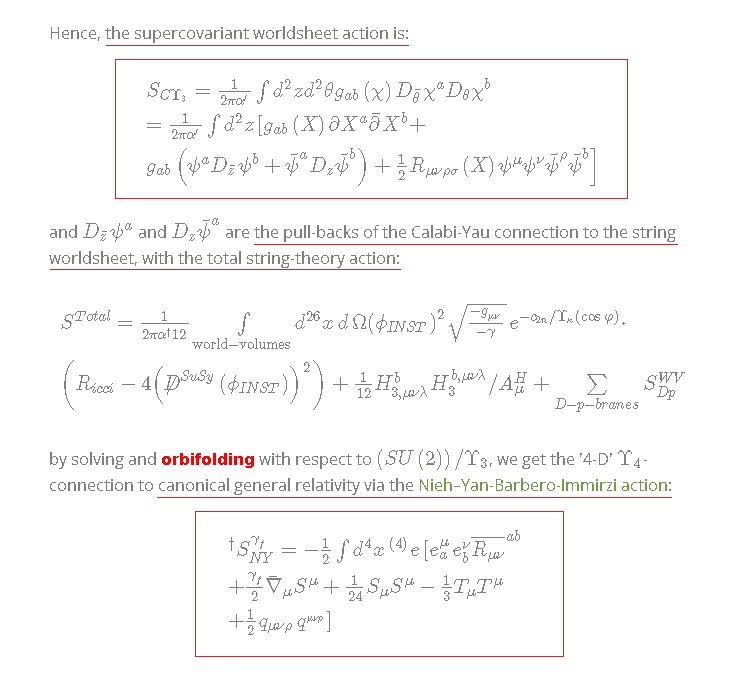
Hence, the supercovariant worldsheet action is:
![\[\begin{array}{l}{S_{C{\Upsilon _3}}} = \frac{1}{{2\pi \alpha '}}\int {{d^2}} z{d^2}\theta {g_{ab}}\left( \chi \right){D_{\bar \theta }}{\chi ^a}{D_\theta }{\chi ^b}\\ = \frac{1}{{2\pi \alpha '}}\int {{d^2}} z\left[ {{g_{ab}}\left( X \right)} \right.\partial {X^a}\bar \partial {X^b} + \\{g_{ab}}\left( {{\psi ^a}{D_{\bar z}}{\psi ^b} + {{\tilde \psi }^a}{D_z}{{\tilde \psi }^b}} \right) + \frac{1}{2}{R_{\mu \nu \rho \sigma }}\left( X \right)\left. {{\psi ^\mu }{\psi ^\nu }{{\tilde \psi }^\rho }{{\tilde \psi }^b}} \right]\end{array}\]](https://www.georgeshiber.com/wp-content/ql-cache/quicklatex.com-f2c9bc07915a1402a1796178a5ece6b2_l3.png "Rendered by QuickLaTeX.com")
and  and
and  are the pull-backs of the Calabi-Yau connection to the string worldsheet, with the total string-theory action:
![\[\begin{array}{l}{S^{Total}} = \frac{1}{{2\pi {\alpha ^\dagger }12}}\int\limits_{{\rm{world - volumes}}} {{d^{26}}} x\,d\,\Omega {\left( {{\phi _{INST}}} \right)^2}\sqrt {\frac{{ - {g_{\mu \nu }}}}{{ - \gamma }}} \,{e^{ - {c_{2n}}/{\Upsilon _\kappa }(\cos \varphi )}} \cdot \\\left( {{R_{icci}} - 4{{\left( {{{\not D}^{SuSy}}\left( {{\phi _{INST}}} \right)} \right)}^2}} \right) + \frac{1}{{12}}H_{3,\mu \nu \lambda }^bH_3^{b,\mu \nu \lambda }/A_\mu ^H + \sum\limits_{D - p - branes} {S_{Dp}^{WV}} \end{array}\]](https://www.georgeshiber.com/wp-content/ql-cache/quicklatex.com-ee1ece1964f54af749ce713bc472b175_l3.png "Rendered by QuickLaTeX.com")
By solving and orbifolding with respect to  , we get the 4-D -connection to canonical general relativity via the Nieh–Yan-Barbero-Immirzi action:
![\[\begin{array}{l}^\dagger S_{NY}^{{\gamma _f}} = - \frac{1}{2}\int {{d^4}} x{\,^{(4)}}e\left[ {e_a^\mu } \right.e_b^\nu {\overline {{R_{\mu \nu }}} ^{ab}}\\ + \frac{{{\gamma _f}}}{2}{{\bar \nabla }_\mu }{S^\mu } + \frac{1}{{24}}{S_\mu }{S^\mu } - \frac{1}{3}{T_\mu }{T^\mu }\\ + \frac{1}{2}{q_{\mu \nu \rho }}\left. {{q^{_{\mu \nu \rho }}}} \right]\end{array}\]](https://www.georgeshiber.com/wp-content/ql-cache/quicklatex.com-bc212042223899729c5ef767c74a794d_l3.png "Rendered by QuickLaTeX.com")
whose isomorphism-class is equivalent to that of general relativity.
The key to the derivation is that  vanishes on hypersurfaces of and that the following holds:
![\[{G_{\alpha \beta }} = 0\]](https://www.georgeshiber.com/wp-content/ql-cache/quicklatex.com-0e31d31f63648d0cc158732bff4c37eb_l3.png "Rendered by QuickLaTeX.com")