All high mathematics serves to do is to beget higher mathematics. ~ Ashim Shanker!
Mathematics is not a careful march down a well-cleared highway, but a journey into a strange wilderness, where the explorers often get lost. Rigour should be a signal to the historian that the maps have been made, and the real explorers have gone elsewhere. W. S. Anglin, in Mathematics and History
In my last post I showed via AdS/CFT analysis, that gravity is an emergent holographic notion: namely, that one can holographically derive (logically deduce) gravity from conformal field theoretic entropic properties of quantum entanglement, and that such a property is a necessary condition for the ‘bundle’ existence of the gravitonic field. To do so, I had to deform CFT by source-fields via the addition of  , which is a dual AdS theory with a bundle field
  and a boundary condition
![\[{J^{\Delta - d + k}} = {J_{CFT}}\]](https://www.georgeshiber.com/wp-content/ql-cache/quicklatex.com-52cd220df35080f7593a28db695f2c6b_l3.png "Rendered by QuickLaTeX.com")
with  the conformal dimension, a local operator
  and
and  equals the number of indices of substracting the contravariant ones to get the AdS/CFT quasi-isomorphic Maldacena correspondence ( = AdS/CFT correspondence), thus the identity
![\[\begin{array}{c}{\left\langle {\Im \{ \exp (\int {{d^4}x{J_{4D}}(X)\vartheta (x))\} } } \right\rangle _{CFT}} = \\{Z_{AdS}}\left[ {\frac{{\lim }}{{boundary}}J{\omega ^{\Delta - d + k}} = {J_{4D}}} \right]\end{array}\]](https://www.georgeshiber.com/wp-content/ql-cache/quicklatex.com-37a60d6a79567a43197d72194a223357_l3.png "Rendered by QuickLaTeX.com")
with the left-hand side being the vacuum expectation value of the time-ordered exponential of the operator over CFT, the right-hand side being the quantum gravity functional with topological-conformal boundary condition, thus leading to holographic emergence, and in a sense, elimination, of gravity. Recall that the Heisenberg Uncertainty Relation holds for energy and time, leading to many anomalies for the Green‘s function of string-propagation:
![\[G({X_{{\sigma _t}(a)}},{X_{{\sigma _t}(b)}}) = \int {{}^sD\exp \left( { - \int_{{\sigma _t}(b)}^{{\sigma _t}(a)} {d{\sigma _t}\int_0^\pi {d{\sigma _t}} } } \right)} \,L\]](https://www.georgeshiber.com/wp-content/ql-cache/quicklatex.com-eede9d9b6212669db1ed3d34d8114ee9_l3.png "Rendered by QuickLaTeX.com")
with  the Lagragian, due to the fact the
  superpositionality with respect to energy makes Feynman path-summation:
![\[P = \frac{\sum }{{{\rm{Topologies}}}}d\mu {\prod _{\mu {\sigma _s}\,{\sigma _t}}}d{X_\mu }({\sigma _s},{\sigma _t})\]](https://www.georgeshiber.com/wp-content/ql-cache/quicklatex.com-bb602098835514aa87fd2eb87d4f0c99_l3.png "Rendered by QuickLaTeX.com")
incoherent since some topologies will degenerate and violate existence conditions for tangent bundles over Minkowski spacetime and some will not correspond to the categorical CFT-manifold, and hence we need to replace the Green’s function with the Källén–Lehmann spectral representation. This is where the GKP-Witten Relation enters with all its glory:
![\[{Z_{CFT}} = {e^{ - S{\,_{GRAVITY}}}}({\phi _i})\]](https://www.georgeshiber.com/wp-content/ql-cache/quicklatex.com-eee7ee020f3ead2034f292915cc80020_l3.png "Rendered by QuickLaTeX.com")
with background deficit angle  and the curvature localized on the boundary with an angular deficit:
![\[R = 4\pi (n - 1) \cdot \delta ({\gamma _A}) + ...\,{\rm{regular terms}}\]](https://www.georgeshiber.com/wp-content/ql-cache/quicklatex.com-4fab363445cb27ed1ffff76a7d7783e7_l3.png "Rendered by QuickLaTeX.com")
with action
![\[\begin{array}{c}{S_A} = \frac{1}{{16\pi {G_N}}}\int {d{x^{d + 2}}} \sqrt g R + \to \\{\rm{Area}}\frac{{({\gamma _A})}}{{4{G_N}}} \cdot (n - 1)\end{array}\]](https://www.georgeshiber.com/wp-content/ql-cache/quicklatex.com-42288341570bc8ef38387d42f8ff563e_l3.png "Rendered by QuickLaTeX.com")
giving us
![\[\begin{array}{*{20}{c}}{{S_A} = \frac{\partial }{{{\partial _n}}}{\rm{log}}{\mkern 1mu} {\rm{T}}{{\rm{r}}_A}{\mkern 1mu} {\rho ^n} = - \frac{\partial }{{{\partial _n}}}{\rm{log}}\left( {\frac{{{Z_n}}}{{{{\left( {{Z_1}} \right)}^n}}}} \right)}\\\begin{array}{c} = {\rm{Area}}\frac{{\left( {{\gamma _A}} \right)}}{{4{G_N}}} \cdot \\\delta {S_{GRAVITY}} = 0 \to {\gamma _A} = {\rm{ minimal surface!}}\end{array}\end{array}\]](https://www.georgeshiber.com/wp-content/ql-cache/quicklatex.com-1d9aa587ca824a160f60615555b8b32a_l3.png "Rendered by QuickLaTeX.com")
with
![\[{S_{GRAVITY}} = \frac{1}{{16\pi {G_N}}}\int {d{x^{d + 2}}} \sqrt {{g_{\mu \nu }}} R + ... \to \frac{{{\rm{Area(}}{\gamma _A})}}{{4{G_N}}} \cdot (n - 1)\]](https://www.georgeshiber.com/wp-content/ql-cache/quicklatex.com-fb3b1de510880d36f3aca28cab1386f1_l3.png "Rendered by QuickLaTeX.com")
hence solving the ‘Ricci/dilaton’ problem I discussed in my last post, since now the holographic formula is
![\[{S_A} = \frac{{\left| {{\gamma _A}} \right|}}{{4G_N^3}} = \frac{c}{3}{\rm{log}}\left( {\frac{{{l_s}}}{a}} \right)\]](https://www.georgeshiber.com/wp-content/ql-cache/quicklatex.com-ef011dbe9b217ad0eb037aec9b13b1b1_l3.png "Rendered by QuickLaTeX.com")
with the ‘magical’ expression ( being the string lenght):
![\[c = \frac{{3R}}{{2G_N^{(3)}}}\]](https://www.georgeshiber.com/wp-content/ql-cache/quicklatex.com-ecacb399c4da1f2f7c552a91a4370db5_l3.png "Rendered by QuickLaTeX.com")
and with that, the GKP-Witten relation solves the ‘Ricci/dilaton’ problem for the action of supergravity theory.
Now let me set up the mathematical context needed to show, in a forthcoming post, that even in M-Theory, or for that matter: any quantum-gravity theory, one cannot coherently quantize gravity in a way that satisfies General Relativistic ‘necessity-criteria’ – as I will show that this would imply, via gravitonic quantum entanglement, the point-‘instantaneous’ collapse of spacetime to a zero-dimensional point like singularity. Not a pretty picture! To do that I have to show that boundary AdS/CFT admits of a ‘local’ symmetry in the bulk theory that is dual to a ‘global’ symmetry corresponding to the boundary and that the (Gubser-Klebanov-Polyakov)-Witten relation deduces the Green correlation functions and that they must have negative Källén–Lehmann spectral representation
![\[\Delta (p) = \int_0^\infty {d{\mu ^2}} \rho ({\mu ^2})\frac{1}{{{p^2} - {\mu ^2} + i\varepsilon }}\]](https://www.georgeshiber.com/wp-content/ql-cache/quicklatex.com-03f1e104d3b09bd0f39e39a17e3d140e_l3.png "Rendered by QuickLaTeX.com")
with  being the gauge-theoretic positive-definite spectral density function.
In the AdS/CFT duality, one must note that the second derivative of the on-shell action principle with respect to the bulk  second-quantized field, must, by unitarity, be identical to the Green function of the current
![\[\begin{array}{c}1.\quad {\left. {\frac{{{\delta ^2}{S_{CFT}}}}{{\delta {A_\mu }(x)\delta A\nu (x')}}} \right|_{u = 0}}\\ \to {G^{\mu \nu }}(x - x') = - {\left\langle {{T_E}{J^\mu }(x){J^\nu }(x')} \right\rangle _G}\end{array}\]](https://www.georgeshiber.com/wp-content/ql-cache/quicklatex.com-a20856c163bcf93b6e1ff3aa76e7ae1e_l3.png "Rendered by QuickLaTeX.com")
with  being the Euclidean time-ordering, and
  the Green function.
For equation 1. to be true, the connected Green function  should provably reduce to the static response function
  in the stationary limit of the following ‘identity’ 2.
![\[2.\quad \mathop {{K^{ij}}}\limits^\_ (k) \equiv {(2\pi )^{p + 1}}{\left. {\frac{{{\delta ^2}_{CFT}}}{{\delta A_i^\dagger ( - k)\delta A_i^\dagger (k)}}} \right|_{u = 0}}\]](https://www.georgeshiber.com/wp-content/ql-cache/quicklatex.com-62286c0e9d56f59f6b0f6eb0f6ba6fe4_l3.png "Rendered by QuickLaTeX.com")
thus, from the limit, one gets the conjectural equation
![\[3.\quad \mathop {{K^{ij}}}\limits^ - (k)\mathop = \limits^? \mathop {{G^{ij}}}\limits^ - (\omega = 0,k)\]](https://www.georgeshiber.com/wp-content/ql-cache/quicklatex.com-bfea1478193d85049887547b480d461b_l3.png "Rendered by QuickLaTeX.com")
But this cannot be true since the holographic Källén–Lehmann spectral representation implies that
![\[\mathop {{K^{ij}}}\limits^ - (k) > 0\]](https://www.georgeshiber.com/wp-content/ql-cache/quicklatex.com-8b1438b9faa008cf5f79195f9647c2bc_l3.png "Rendered by QuickLaTeX.com")
whereas 
Now, the definite-negativeness of  can be derived from the Källén–Lehmann spectral representation of the ‘connected’ Green function:
![\[4.\quad \mathop {{G^{\mu \nu }}}\limits^ - ({\omega _n},k) = \int_{ - \infty }^\infty {\frac{{d\omega }}{{2\pi }}} \frac{{\mathop {{\rho ^{\mu \nu }}(\omega ,k)}\limits^ - }}{{i{\omega _n} - \omega }}\]](https://www.georgeshiber.com/wp-content/ql-cache/quicklatex.com-0ab78894e208f8718de7191a6d2e0bc9_l3.png "Rendered by QuickLaTeX.com")
where  must be the Matsubara frequencies and
  is a Fourier spectral functional transform of:
![\[5.\quad {\rho ^{\mu \nu }}(t,x) \equiv \left\langle {\left[ {{J^\mu }(t,x),{J^\nu }(0,0)} \right]} \right\rangle \]](https://www.georgeshiber.com/wp-content/ql-cache/quicklatex.com-64f2b0a62cf261f607e32ac52468fef8_l3.png "Rendered by QuickLaTeX.com")
However, this spectral function satisfies
![\[\mathop {{\rho ^{\mu \mu }}}\limits^ - (\omega ,k)/\omega > 0\]](https://www.georgeshiber.com/wp-content/ql-cache/quicklatex.com-732b3b067300891a7292f516837e7982_l3.png "Rendered by QuickLaTeX.com")
thus leading to the definite-negativeness of:
![\[6.\quad \mathop {{G^{ii}}}\limits^ - (o,k) = - \int_{ - \infty }^\infty {\frac{{d\omega }}{{2\pi }}} \frac{{\mathop {{\rho ^{ii}}(\omega ,k)}\limits^ - }}{\omega } < 0\]](https://www.georgeshiber.com/wp-content/ql-cache/quicklatex.com-d6afcfce8c73271c354d5e8b20beb61a_l3.png "Rendered by QuickLaTeX.com")
no ‘summing’ over ‘i’. Because the ‘connected’ Green function and the holographic Källén–Lehmann spectral representational functional differ by a sign,
must be false!
A resolution to this contradiction is obtained by noting that the AdS/CFT bulk theory has gauge symmetry and the boundary theory has background-local symmetry: hence the current  does contain an external source field
  . In such a case, the Källén–Lehmann spectral representational functional can differ from the Green function, and the GKP-Witten relation yields the holographic Källén–Lehmann spectral function instead of the Green function. To show how this works, take a complex scalar field
  coupled to the the electromagnetic field :
![\[\begin{array}{c}{S_A}\left[ \phi \right] = \int {{d^{p + 1}}} x \cdot \\\left( {{{\left| {\left( {{{\not \partial }_\mu } - ie{A_\mu }} \right)} \right|}^2} + V\left( {\left| \phi \right|} \right)} \right)\end{array}\]](https://www.georgeshiber.com/wp-content/ql-cache/quicklatex.com-8ea0a623ec6705cc28addbe204ad5f03_l3.png "Rendered by QuickLaTeX.com")
Now, the current
![\[7.\quad {J^\mu } = - \frac{{\delta {S_A}}}{{\delta {A_\mu }}} = - ie{\phi ^\dagger }\mathop {{\partial ^\mu }}\limits^ \leftrightarrow \phi - 2{e^2}{A^\mu }{\left| \phi \right|^2}\]](https://www.georgeshiber.com/wp-content/ql-cache/quicklatex.com-d96d8f82b637a3bd4d4fe9ca12ad5af9_l3.png "Rendered by QuickLaTeX.com")
contains the electromagnetic field by the background local symmetry. Now, one can generate the functional
![\[8.\quad Z{\rm{[}}A{\rm{]}} = {e^{W{\rm{[}}A{\rm{]}}}} = \int {D{\phi ^\dagger }} D{\phi ^{ - {S_A}{\rm{[}}\phi {\rm{]}}}}\]](https://www.georgeshiber.com/wp-content/ql-cache/quicklatex.com-1c60ede366bde978121b9c979e0f1206_l3.png "Rendered by QuickLaTeX.com")
thus deriving the current expectation value as
![\[9.\quad \left\langle {{J^\mu }} \right\rangle = - \left\langle {\frac{{\delta {S_A}}}{{\delta {A_\mu }}}} \right\rangle = \frac{{\delta W{\rm{[}}A{\rm{]}}}}{{\delta {A_\mu }}}\]](https://www.georgeshiber.com/wp-content/ql-cache/quicklatex.com-051b9be36367bde944a0b17321914d63_l3.png "Rendered by QuickLaTeX.com")
with a ‘response’ functional
![\[{K^{\mu \nu }}\]](https://www.georgeshiber.com/wp-content/ql-cache/quicklatex.com-d013e87409f50ea6ca6c9de1ddfcc98d_l3.png "Rendered by QuickLaTeX.com")
given by
![\[\begin{array}{c}10.\quad {K^{\mu \nu }}(x): = - \frac{{\delta \left\langle {{J^\mu }(x)} \right\rangle }}{{\delta {A_\nu }(0)}} = - \frac{{{\delta ^2}W{\rm{[}}A{\rm{]}}}}{{\delta {A_\nu }(0)\delta {A_\mu }(x)}}\\ = {G^{\mu \nu }}(x) - \left\langle {\frac{{\delta {J^\mu }(x)}}{{\delta {A_\nu }(0)}}} \right\rangle \\ = {G^{\mu \nu }}(x) + 2{e^2}{\delta ^{\mu \nu }}\delta (x)\left\langle {{{\left| {\phi (x)} \right|}^2}} \right\rangle \end{array}\]](https://www.georgeshiber.com/wp-content/ql-cache/quicklatex.com-06dc3031a5cf367eb782af9e87859a14_l3.png "Rendered by QuickLaTeX.com")
where  is the ‘connected’ Green function for the current
![\[\begin{array}{c}11.\quad {G^{\mu \nu }}(x) = \\ - {\left\langle {{T_E}{J^\mu }(x){J^\nu }(0)} \right\rangle _G}\end{array}\]](https://www.georgeshiber.com/wp-content/ql-cache/quicklatex.com-2a65f964258cddeb768dc820ecc0ef75_l3.png "Rendered by QuickLaTeX.com")
Therefore, the Källén–Lehmann spectral representation functional differs from the ‘connected’ Green function by the second term of
![\[{G^{\mu \nu }}(x) + 2{e^2}{\delta ^{\mu \nu }}\delta (x)\left\langle {{{\left| {\phi (x)} \right|}^2}} \right\rangle \]](https://www.georgeshiber.com/wp-content/ql-cache/quicklatex.com-5670f4cd0d7a3dc750f4f4e8866c979e_l3.png "Rendered by QuickLaTeX.com")
Hence, the ‘negativity’ is not reflected in the Källén–Lehmann spectral representation functional and from
one gets the GKP-Witten relational implication:
![\[{A_\mu } = 0\]](https://www.georgeshiber.com/wp-content/ql-cache/quicklatex.com-b9aa5c519d2fd0de116178c52c570410_l3.png "Rendered by QuickLaTeX.com")
Applied in a forthcoming post to the quantum gravitational field
![\[Q_\mu ^{{G_{ST}}}(R_{{S_{({\sigma _s},{\sigma _t})}}}^{2d})\]](https://www.georgeshiber.com/wp-content/ql-cache/quicklatex.com-dfcad95bf94097d52864ed3d1660caec_l3.png "Rendered by QuickLaTeX.com")
I will derive, via quantum entanglement and gravitonic vacuua analysis, the collapse of spacetime to a zero-dimensional point-like singularity that also violates the Theory of Special Relativity (in fact, what will it not violate), and the GKP-Witten Relation will be central in that analysis. Note: the AdS/CFT holography principle entropically implies the ’emergence’-property, and thus quantum-field-theoretic elimination, of the gravitational field.