Loop Quantum Cosmology and the Wigner-Moyal-Groenewold Phase Space

By George Shiber Wednesday, March 1, 2017Saturday, August 17, 2019 In Cosmology, Loop Quantum Gravity, Mathematical Physics, Mathematics, Philosophy Of Physics, Philosophy Of Science, Physics Loop Quantum Cosmology, quantum gravity

I will derive a crucial property of loop quantum cosmology it shares with string/M-theory and asymptotically free quantum gravity theory, namely, that the associated Wigner-Moyal-Groenewold operator-formalism entails that the Holst-Barbero-Immirzi 4-spinfold has the property of spacetime uncertainty that I derived for string/M-theory, an essential property if loop quantum gravity is to be a valid quantum gravity theory. As I showed, in 4-D spacetime, the general relativistic starting point for canonical loop quantum gravity is given by:

$\begin{array}{l}{S_{4{\rm{D}}}}\left[ {e',\omega } \right] = \int_{\tilde M} {\left( {\frac{1}{2}} \right.} {\rm{tr}}\left( {e \wedge e \wedge F} \right)\\\left. { + \frac{1}{\gamma }{\rm{tr}}\left( {e \wedge e \wedge * F} \right)} \right)\end{array}$

where the dynamical variables are the tetrad one-form fields:

${e^I} = e_\mu ^I{\rm{d}}{x^\mu }$

and the $SL\left( {2,\mathbb{C}} \right)$ -valued connection $\omega _\mu ^{IJ}$ whose curvature is:

$F = {\rm{d}}\omega + \omega \wedge '\omega$

and is a connection on the holonomy-flux algebra for a homogeneous isotropic Friedmann–Lemaître–Robertson–Walker ‘space’

Hence, we have the two-form:

$\begin{array}{l}{F^{IJ}} = \left( {{{\not \partial }_\mu }} \right.\omega _\nu ^{IJ} - {{\not \partial }_\nu }\omega _\mu ^{IJ} + \omega _\mu ^{IK}{\omega _\nu }{K^J}\\\left. { - \omega _\nu ^{IK}{\omega _\mu }{K^J}} \right){\rm{d}}{x^\mu } \wedge '{\rm{d}}{x^\nu }\end{array}$

with:

$* {F^{IJ}} = \frac{1}{2}{\varepsilon ^{IJ}}_{KL}{F^{KL}}$

and ${\rm{Tr}}$ is the Killing form on the Lie algebra $SL\left( {2,\mathbb{C}} \right)$ :

${\rm{Tr}}\left( {e \wedge e \wedge F} \right) = {\varepsilon _{IJKL}}{e^I} \wedge {e^J}{F^{KL}}$

with

${\varepsilon _{IJKL}}$

the totally antisymmetric tensor given by:

${\varepsilon ^{0123}} = + 1$

Now, I can write down the Holst action more informatively:

$\begin{array}{*{20}{l}}{{S_{4D}}\left[ {e,\omega } \right] = \int_{{{\tilde M}_4}} {{{\rm{d}}^4}} x{\varepsilon ^{\mu \nu \rho \sigma }}\left( {\frac{1}{2}} \right.{\varepsilon _{IJKL}}}\\{e_\mu ^Ie_\nu ^JF_{\rho \sigma }^{KL}\left. { + \frac{1}{\gamma }e_\mu ^Ie_\nu ^J{F_{\rho \sigma }}_{IJ}} \right)}\end{array}$

and from the Ashtekar variables, our action is:

${{S_H} = \int {{d^3}} x\left\{ {{{\tilde E}^a}_B\dot A_a^B - \frac{1}{2}{\omega _{aBC}}{\varepsilon ^{BCD}}{t^a}{G_D} - {N^a}{C_a} - NH} \right\}}$

${\left\{ {A_a^B\left( x \right),\tilde E_A^b\left( y \right)} \right\} = \delta _a^b\delta _A^B\delta \left( {x,y} \right)}$

with the Gaussian constraint:

${G_A} = {D_a}{\tilde E^a}A$

the diffeomorphism constraint:

${C_a} = {\tilde E^b}{F_{ab}}^A + \frac{{\left( {1 + {\gamma ^2}} \right)}}{\gamma }{K_a}^A{G_A}$

and our Hamiltonian is given by:

$H = \frac{{8\pi G{\gamma ^2}}}{{\sqrt {\left| {\det \left( q \right)} \right|} }}{\tilde E^a}_A{\tilde E^b}_B\left[ {{\varepsilon ^{AB}}_C{F_{ab}}^C - \frac{{2\left( {1 + {\gamma ^2}} \right)}}{\gamma }{K_a}^A{K_b}^B} \right]$

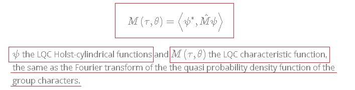
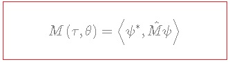
The LQC Wigner-Moyal-Groenewold operator is the unique operator with the following properties:

$M\left( {\tau ,\theta } \right) = \left\langle {{\psi ^ * },\hat M\psi } \right\rangle$

$\psi$ the LQC Holst-cylindrical functions and $M\left( {\tau ,\theta } \right)$ the LQC characteristic function, the same as the Fourier transform of the the quasi probability density function of the group characters.

It immediately follows from Fourier phase space symplecticity that the LQC Wigner-Moyal-Groenewold operator satisfies the following relation:

${\hat M\left( {\tau ,\theta } \right) = {e^{i\frac{\tau }{a}\hat p}}{{\hat h}_\theta }{e^{i\frac{\tau }{a}\hat p}} = {e^{i\frac{\tau }{a}\hat p}}{e^{i\theta c}}{e^{i\frac{\tau }{a}\hat p}}}$

${\hat p \equiv - ia\frac{d}{{dc}}}$

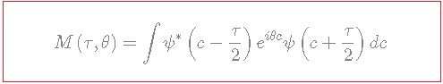
and for the LQC characteristic function, we have:

$M\left( {\tau ,\theta } \right) = \int {{\psi ^ * }} \left( {c - \frac{\tau }{2}} \right){e^{i\theta c}}\psi \left( {c + \frac{\tau }{2}} \right)dc$

noting that any connection $c$ is gauge and diffeomorphism invariant in homogeneous isotropic space.

We can now define the holonomy-flux algebra for homogeneous isotropic Friedmann–Lemaître–Robertson–Walker space model via:

$\left[ {{{\hat N}_{\left( \mu \right)}},\hat p} \right] = - \frac{{8\pi G\hbar }}{3}\mu {\hat N_{\left( \mu \right)}}$

where the holonomy and the flux operators act as:

${{\hat N}_{\left( \mu \right)}}\Psi \left( c \right) = {e^{i\mu c}}$

$\hat p\Psi \left( c \right) = - i\frac{{8\pi \gamma G\hbar }}{3}\frac{{d\Psi }}{{dc}}$

The Hilbert space basis is given by the connection-lifter LQG spin-networks:

${\hat N_{\left( \mu \right)}} = {e^{i\mu c}}$

with $c$ the configuration variable corresponding to the connection, $\mu$ the number of the Fourier fiducial cell repetition, and satisfy:

$\left\langle {{N_{\left( \mu \right)}},{N_{\mu '}}} \right\rangle = \left\langle {{e^{i\mu c}}{e^{i\mu 'c}}} \right\rangle = {\delta _{\mu ,\mu '}}$

and:

$\left[ {\hat p,\hat N} \right] = a\mu \hat N$

with $a$ a constant satisfying:

$a = \frac{{4\pi \gamma G\hbar }}{3}$

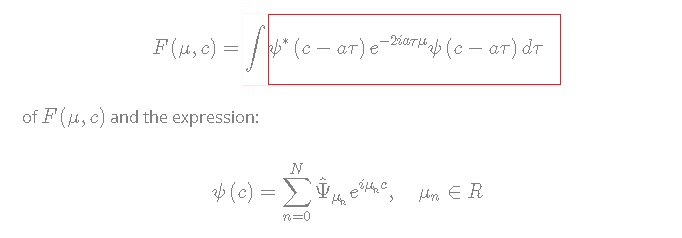
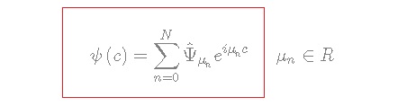
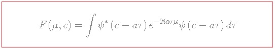
Let us derive now the Wigner function and show that it satisfies the property that when integrated by one variable it reduces to the distribution density of the other variable. Define it as:

$F\left( {\mu ,c} \right) = \int {{\psi ^ * }} \left( {c - a\tau } \right){e^{ - 2ia\tau \mu }}\psi \left( {c - a\tau } \right)d\tau$

with:

$\psi \left( c \right) = \sum\limits_{n = 0}^N {{{\hat \Psi }_{{\mu _n}}}{e^{i{\mu _n}c}}} ,\quad {\mu _n} \in R$

For the distribution density function to be definable, the mutual quasi distribution function of $\mu$ and $c$ the following two equalities should be true:

${\rho _c} = \int {F\left( {\mu ,c} \right)} \,dc = {\left| {\psi \left( c \right)} \right|^2}$

${\rho _\mu } = \int {F\left( {\mu ,c} \right)} \,dc = {\left| {\hat \Psi \left( c \right)} \right|^2}$

Hence, when integrating with respect to one variable it becomes the distribution density of the other one. The above equalities hold since our measures $dc$ and $d\mu$ satisfy:

$\int\limits_{{{\hat R}_b}} {{{\hat f}_\mu }d\mu } = \sum\limits_{\mu \in R} {{{\hat f}_\mu }}$

and:

$\int\limits_{{R_b}} {{e^{i\mu c}}} dc = {\delta _{\mu ,0}}$

with ${\hat R_b}$ the Bohr dual space and ${\delta _{\mu ,0}}$ a Kronecker delta.

Now, the characters of the compactified line ${R_b}$ are the functions ${h_\mu }\left( c \right) = {e^{i\mu c}}$ , hence the Fourier transform of the function on ${R_b}$ is given by:

${\hat f_\mu } = \int {f\left( c \right)} {h_{ - \mu }}\left( c \right)dc$

which is an isomorphism of:

${L^2}\left( {{R_b},c} \right) \to {L^2}\left( {{{\hat R}_b},d\mu } \right)$

and ${e^{i\mu c}}$ comprise the basis of:

$H = {L^2}\left( {{R_b},dc} \right)$

We need to prove the above equalities. First, substitute the expression:

$F\left( {\mu ,c} \right) = \int {{\psi ^ * }} \left( {c - a\tau } \right){e^{ - 2ia\tau \mu }}\psi \left( {c - a\tau } \right)d\tau$

of $F\left( {\mu ,c} \right)$ and the expression:

$\psi \left( c \right) = \sum\limits_{n = 0}^N {{{\hat \Psi }_{{\mu _n}}}{e^{i{\mu _n}c}}} ,\quad {\mu _n} \in R$

for $\psi \left( c \right)$ into:

${\rho _c} = \int {F\left( {\mu ,c} \right)} \,dc = {\left| {\psi \left( c \right)} \right|^2}$

giving us:

$\begin{array}{l}\int {F\left( {\mu ,c} \right)} \,d\mu = \int {\int {\sum\limits_{n = 0}^N {\sum\limits_{k = 0}^K {\hat \Psi _{{\mu _n}}^ * } } } } {e^{ - ia{\mu _n}c}}\\{e^{ia{\mu _n}\tau }}{{\hat \Psi }_{{\mu _k}}}{e^{ia{\mu _k}c}}{e^{ia{\mu _k}\tau }}{e^{ - 2ia\tau \mu }}d\tau d\mu \end{array}$

with $\tau \in {R_b},\;\mu \in R$ , and since integration with respect to $\mu$ is just a sum as $\mu$ is discrete, we have:

$\begin{array}{l}\int {F\left( {\mu ,c} \right)} \,d\mu = \sum\limits_{\mu \in R} {\sum\limits_{n = 0}^N {\sum\limits_{k = 0}^K {\int {\hat \Psi _{{\mu _n}}^ * } } } } {e^{ - ia{\mu _n}c}}\\{e^{ia{\mu _n}\tau }}{{\hat \Psi }_{{\mu _n}}}{e^{ia{\mu _n}c}}{e^{ia{\mu _n}\tau }}{e^{ - 2ia\tau \mu }}d\tau \end{array}$

Now, using:

$\int\limits_{{R_b}} {{e^{i\mu c}}} dc = {\delta _{\mu ,0}}$

and integrating with respect to $\tau$ , we can derive:

$\int {{e^{ia{\mu _n}\tau }}{{\hat \Psi }_{{\mu _n}}}{e^{ia{\mu _k}\tau }}{e^{ - 2ia\tau \mu }}d\tau } = {\delta _{2\mu ,{\mu _k} + {\mu _n}}}$

Given $\mu \in R$ , it follows that summation by $\mu$ makes the terms with $2\mu \ne {\mu _k} + {\mu _n}$ equal to zero and the terms with $\mu = {\mu _k} + {\mu _n}$ equal to one and all terms with $\tau$ and $\mu$ vanish from the sum. Hence, by using:

$\psi \left( c \right) = \sum\limits_{n = 0}^N {{{\hat \Psi }_{{\mu _n}}}{e^{i{\mu _n}c}}} ,\quad {\mu _n} \in R$

we derive:

$\begin{array}{l}\int {F\left( {\mu ,c} \right)} \,d\mu = \sum\limits_{n = 0}^N {\sum\limits_{k = 0}^K {\hat \Psi _{{\mu _n}}^ * {e^{ - ia{\mu _n}c}}} } \\{{\hat \Psi }_{{\mu _k}}}{e^{ia{\mu _k}c}} = {\psi ^ * }\left( c \right)\psi \left( c \right) = {\left| {{\psi ^ * }\left( c \right)} \right|^2}\end{array}$

and to prove the equality:

${\rho _\mu } = \int {F\left( {\mu ,c} \right)} \,dc = {\left| {\hat \Psi \left( c \right)} \right|^2}$

we substitute the expression:

$\left[ {\hat p,\hat N} \right] = a\mu \hat N$

of ${F\left( {\mu ,c} \right)}$ and the expression:

$\psi \left( c \right) = \sum\limits_{n = 0}^N {{{\hat \Psi }_{{\mu _n}}}{e^{i{\mu _n}c}}} ,\quad {\mu _n} \in R$

for $\psi \left( c \right)$ into it, yielding:

${\int {F\left( {\mu ,c} \right)} {\mkern 1mu} d\mu = \int {\int {\sum\limits_{n = 0}^N {\sum\limits_{k = 0}^K {\hat \Psi _{{\mu _n}}^*{e^{ - ia{\mu _n}c}}{e^{ia{\mu _n}\tau }}} {e^{ - 2ia\tau \mu }}d\tau dc} } } }$

Now, integration with measure $dc$ given:

$\int\limits_{{R_b}} {{e^{i\mu c}}} dc = {\delta _{\mu ,0}}$

yields:

$\int {{e^{ - ia{\mu _n}c}}} {e^{ia{\mu _k}c}}dc = {\delta _{\mu k - \mu n,0}}$

Hence, only the terms with ${\mu _k} = {\mu _n}$ remain in:

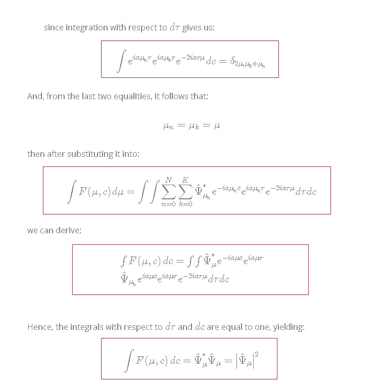
and since integration with respect to $d\tau$ gives us:

$\int {{e^{ia{\mu _n}\tau }}} {e^{ia{\mu _k}\tau }}{e^{ - 2ia\tau \mu }}dc = {\delta _{2\mu ,{\mu _k} + {\mu _n}}}$

And, from the last two equalities, it follows that:

${\mu _n} = {\mu _k} = \mu$

then after substituting it into:

we can derive:

$\begin{array}{l}\int {F\left( {\mu ,c} \right)} \,dc = \int {\int {\hat \Psi _\mu ^ * } } {e^{ - ia\mu c}}{e^{ia\mu \tau }}\\{{\hat \Psi }_{{\mu _n}}}{e^{ia\mu c}}{e^{ia\mu \tau }}{e^{ - 2ia\tau \mu }}d\tau dc\end{array}$

Hence, the integrals with respect to $d\tau$ and $dc$ are equal to one, yielding:

$\int {F\left( {\mu ,c} \right)} \,dc = \hat \Psi _\mu ^ * {\hat \Psi _\mu } = {\left| {{{\hat \Psi }_\mu }} \right|^2}$

So, from:

and:

$\int {F\left( {\mu ,c} \right)} \,dc = \hat \Psi _\mu ^ * {\hat \Psi _\mu } = {\left| {{{\hat \Psi }_\mu }} \right|^2}$

it follows that $F\left( {\mu ,c} \right)$ is a LQC Wigner function in variables $\mu$ , $c$ , completing the proof.

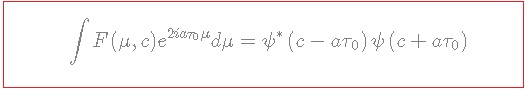
Next, we need to prove that the first momentum has the following property:

$\int {F\left( {\mu ,c} \right)} {e^{2ia{\tau _0}\mu }}d\mu = {\psi ^ * }\left( {c - a{\tau _0}} \right)\psi \left( {c + a{\tau _0}} \right)$

with $c,{\tau _0} \in {R_b}$ . Start with substituting the red area:

into the left-hand-side of:

$\int {F\left( {\mu ,c} \right)} {e^{2ia{\tau _0}\mu }}d\mu = {\psi ^ * }\left( {c - a{\tau _0}} \right)\psi \left( {c + a{\tau _0}} \right)$

yielding:

$\begin{array}{c}\int {F\left( {\mu ,c} \right)\,} {e^{ - 2ia\tau \mu }}d\mu = \int {\int {{\psi ^ * }} } \left( {c - a\tau } \right)\\{e^{2ia{\tau _0}\mu }}\psi \left( {c + a\tau } \right)d\tau d\mu \end{array}$

By using the red-area expression below

for $\psi \left( c \right)$ , we can deduce:

$\begin{array}{*{20}{l}}{\int {F\left( {\mu ,c} \right)} {\mkern 1mu} {e^{2ia{\tau _0}\mu }}d\mu = \int {\int {\sum\limits_{n = 0}^N {\sum\limits_{k = 0}^K {\hat \Psi _{{\mu _n}}^*} } } } {e^{ - ia{\mu _n}c}}{e^{ia{\mu _n}\tau }}}\\{{{\hat \Psi }_{{\mu _k}}}{e^{ia{\mu _k}c}}{e^{ia{\mu _k}\tau }}{e^{ - 2ia\tau \mu }}{e^{2ia{\tau _0}\mu }}d\tau d\mu }\end{array}$

repeating the step above, integrating by $\mu$ can be replaced by summing over $\mu$ :

$\begin{array}{l}\int {F\left( {\mu ,c} \right)} \,{e^{2ia{\tau _0}\mu }}d\mu = \sum\limits_{\mu \in R} {\sum\limits_{n = 0}^N {\sum\limits_{k = 0}^K {\int {\hat \Psi _{{\mu _n}}^ * } } } } {e^{ - ia{\mu _n}c}}{e^{ia{\mu _n}\tau }}\\{{\hat \Psi }_{{\mu _k}}}{e^{ia{\mu _k}c}}{e^{ia{\mu _k}\tau }}{e^{ - 2ia\tau \mu }}{e^{2ia{\tau _0}\mu }}d\tau \end{array}$

and integrating by $\tau$ yields:

$\int {{e^{ia{\mu _n}\tau }}{e^{ia{\mu _k}\tau }}} {e^{ - 2ia\tau \mu }}d\tau = {\delta _{2\mu ,{\mu _k} + {\mu _n}}}$

thus since the sum over $\tau$ equals one, we have:

$\int {F\left( {\mu ,c} \right)} \,{e^{2ia{\tau _0}\mu }}d\mu = \sum\limits_n {\sum\limits_k {\hat \Psi _{{\mu _n}}^ * } } {e^{ - ia{\mu _n}c}}{\hat \Psi _{{\mu _k}}}{e^{ia{\mu _k}c}}{e^{2ia{\tau _0}\mu }}$

substituting $2\mu = {\mu _k} + {\mu _n}$ into it and using the definition of the LQC cylindrical functions:

we get:

$\begin{array}{l}\int {F\left( {\mu ,c} \right)} \,{e^{2ia{\tau _0}\mu }}d\mu = \sum\limits_n {\sum\limits_k {\hat \Psi _{{\mu _n}}^ * } } {e^{ - ia{\mu _n}c}}{{\hat \Psi }_{{\mu _k}}}{e^{ia{\mu _k}c}}{e^{ia{\tau _0}\mu \left( {{\mu _n} + {\mu _k}} \right)}}\\ = {\psi ^ * }\left( {c - a{\tau _0}} \right)\psi \left( {c + a{\tau _0}} \right)\end{array}$

Proving that the first momentum has the desired property:

Now, we need to show that the LQC Wigner-Moyal-Groenewold operator has the following property:

We substitute $F\left( {\mu ,c} \right)$ from:

into:

to obtain:

$M\left( {\tau ,\theta } \right) = \int {\int {\int {{\psi ^ * }} } } \left( {c - a{\tau _0}} \right){e^{ - 2ia{\tau _0}}}\psi \left( {c + a{\tau _0}} \right)d{\tau _0}{e^{i\tau \mu }}{e^{i\theta c}}d\mu dc$

and by utilizing $\psi \left( c \right)$ from our definition:

it reduces to:

$\begin{array}{l}M\left( {\tau ,\theta } \right) = \int {\int {\int {\sum\limits_{n = 0}^N {\sum\limits_{k = 0}^K {\psi _{{\mu _0}}^ * } } } } } {e^{ - i{\mu _0}c}}{e^{ia{\mu _0}{\tau _0}}}\\{{\hat \Psi }_{{\mu _k}}}{e^{ - i{\mu _k}c}}{e^{ia{\mu _k}{\tau _0}}}{e^{ - 2ia{\tau _0}\mu }}d{\tau _0}{e^{i\tau \mu }}{e^{i\theta c}}d\mu dc\end{array}$

The same integration rules applied above go through now as well, yielding:

$M\left( {\tau ,\theta } \right) = \int {\sum\limits_n {\sum\limits_k {\hat \Psi _{{\mu _0}}^ * } } } {e^{ - i{\mu _n}c}}{\hat \Psi _{{\mu _k}}}{e^{i{\mu _k}c}}{e^{i\tau \frac{{\left( {{\mu _k} + {\mu _n}} \right)}}{2}}}{e^{i\theta c}}dc$

Combining the terms in the exponents and using the LQC cylindrical function above, we have:

$\left\{ {\begin{array}{*{20}{c}}{\psi \left( {c - \frac{\tau }{2}} \right)}\\{\psi \left( {c + \frac{\tau }{2}} \right)}\end{array}} \right.$

Hence, we derived the LQC characteristic function $M\left( {\tau ,\theta } \right)$ as a Fourier transform of $F\left( {\mu ,c} \right)$ :

$M\left( {\tau ,\theta } \right) = \int {{\psi ^ * }} \psi \left( {c - \frac{\tau }{2}} \right){e^{i\theta c}}\psi \left( {c + \frac{\tau }{2}} \right)dc$

Now, we must prove that the following operator:

$\hat M\left( {\tau ,\theta } \right) = {e^{i\frac{\tau }{a}\hat p}}{\hat h_\theta }{e^{i\frac{\tau }{a}\hat p}} = {e^{i\frac{\tau }{a}\hat p}}{e^{i\theta c}}{e^{i\frac{\tau }{a}\hat p}}$

is a Wigner-Moyal-Groenewold operator, where:

$\hat p = - ia\frac{d}{{dc}}$

We start by substituting

$\hat M\left( {\tau ,\theta } \right) = {e^{i\frac{\tau }{a}\hat p}}{\hat h_\theta }{e^{i\frac{\tau }{a}\hat p}} = {e^{i\frac{\tau }{a}\hat p}}{e^{i\theta c}}{e^{i\frac{\tau }{a}\hat p}}$

into:

yielding:

$\left\langle {{\psi ^ * },\hat M\psi } \right\rangle = \int {{\psi ^ * }} \left( c \right){e^{i\frac{\tau }{a}\hat p}}{e^{i\theta c}}{e^{i\frac{\tau }{a}\hat p}}\psi \left( c \right)dc$

and expanding the exponents into the Taylor series allows us to derive:

$\begin{array}{l}\left\langle {{\psi ^ * },\hat M\psi } \right\rangle = \int {{\psi ^ * }} \left( c \right)\left( {1 + \frac{{i\tau }}{{2a}}\left( { - ia\frac{d}{{dc}} + ...} \right){e^{i\theta c}}} \right)\\\left( {1 + \frac{{i\tau }}{{2a}}\left( { - ia\frac{d}{{dc}} + ...} \right)\psi \left( c \right)dc} \right) = \int {{\psi ^ * }\left( {c - \frac{\tau }{2}} \right)} \,\psi \left( {c + \frac{\tau }{2}} \right)dc = M\left( {\tau ,\theta } \right)\end{array}$

amounting to a proof that:

$\hat M\left( {\tau ,\theta } \right) = {e^{i\frac{\tau }{a}\hat p}}{\hat h_\theta }{e^{i\frac{\tau }{a}\hat p}} = {e^{i\frac{\tau }{a}\hat p}}{e^{i\theta c}}{e^{i\frac{\tau }{a}\hat p}}$

is a Wigner-Moyal-Groenewold operator for a homogeneous and isotropic space whose connection-form is gauge and diffeomorphism invariant, and by the symplecticity of the associated LQG holonomy-flux algebra, the Holst-Barbero-Immirzi 4-spinfold has the property of space-time uncertainty:

$\Delta {T_{bar}}\Delta {X_{imri}} \ge \ell _{LQG}^2$

with:

$\left\{ {\begin{array}{*{20}{c}}{\Delta {X_{imri}} \sim g_{LQG}^{1/3}{\ell _{LQG}}}\\{\Delta {T_{bar}} \sim g_{LQG}^{ - 1/3}{\ell _{LQG}}}\end{array}} \right.$