M-Theory, Kaluza-Klein Splitting, U-Duality and F-Theory

By George Shiber Sunday, April 16, 2017Friday, October 26, 2018 In F Theory, M Theory, Mathematical Physics, Mathematics, Physics F-Theory, Kaluza-Klein Splitting

There is a deep connection between the U-duality groups of M-theory and the embedding of the 11-dimensions in the extended superspace which under the gauge and diffeomorphism group actions, induces a continuous ${E_{d(d)}}$ symmetry. Here, I will relate the F-theory action to that of M-theory in the context of the F-theory/M-theory duality with an ${\rm{SL}}\left( N \right) \times {\mathbb{R}^ + }$ representation. Recall that F-theory is a one-time theory, so let us start with how to make a space-like brane time-like in M-theory. Keeping in mind that the total action of M-theory is given by:

$\begin{array}{*{20}{l}}{{S_M} = \frac{1}{{{k^9}}}\int\limits_{world - vol} {{d^{11}}} \sqrt {\frac{{ - {g_{\mu \nu }}}}{{ - \gamma }}} T_p^{10}d\Omega {{\left( {{\phi _{Inst}}} \right)}^{26}}\left( {{R_{icci}} - A_\mu ^H\frac{1}{{48}}G_4^2} \right)}\\{ + \sum\limits_{Dp} {D_\mu ^S} {e^{ - H_3^b}}/S_{Dp}^{WV} + \sum\limits_{Dp} {D_\mu ^S} {e^{ - H_3^b}}/{S^{Total}}}\end{array}$

as I showed here, with ${T_p} \sim {\alpha ^\dagger }\frac{{p + 1}}{2}$ the D-p-brane world-volume tension, and the Yang-Mills field strength being:

${F_{\mu \nu }} = {\partial _\mu }A_\mu ^H - {\partial _\nu }\bar A_\mu ^H + \left[ {A_\mu ^H,\Upsilon _{2\kappa }^i(\cos \varphi )} \right]$

and by a Paton-Chern-Simons factor, we get:

$\left[ {A_\mu ^H,A_\nu ^H} \right] = \sum\limits_{k = 1}^N {A_\mu ^{H,ac}} A_\nu ^{H,cb} - A_\nu ^{H,ac}A_\mu ^{H,cb}$

${\phi _{Inst}}$ the instanton field, with:

${e^{ - {\phi _{Inst}}{g_{\mu \nu }}}} = {e^{ - 2{\phi _{Inst}}\left( {{g_{\mu \nu }} - 1} \right)}}$

and ${g_{\mu \nu }} = {e^{{{\left( {{\phi _{Inst}}} \right)}^2}}}$ .

Space-like branes are a class of time-dependent solutions of M-theory with topological defects localized in (P + 1)-dimensional space-like surfaces and exist at a moment in time, and are time-like super-tachyonic kink solutions of unstable D(P + 1)-branes in string theory and provide the topology of the throat-bulk. Let us start with a Dp-Dp pair Lagrangian, fixing the boundary of the string field theory superspace, so that the action is:

$S = {\mkern 1mu} - 2{T_{D9}}\int {{d^{10}}} x{e^{ - \pi {{\left| T \right|}^2}}}F\left( {X + \sqrt Y } \right)F\left( {X - \sqrt Y } \right)$

with

$\left\{ {\begin{array}{*{20}{c}}{X \equiv {\partial _\mu }T{\partial ^\mu }\bar T}\\{Y \equiv {{\left( {{\partial _\mu }T} \right)}^2}{{\left( {{\partial ^\nu }\bar T} \right)}^2}}\end{array}} \right.\quad p = 9$

and

$T = {T_{cl(st)}}(x) = x + \sum\limits_{cl{{(st)}_x}} {\int_{cl{{(st)}_x}} {{e^{\tilde T(x)}}} } \gg 0$

A Teichmuller BPS D(P+1)-brane 2-D reduction gives us the throat action:

$S = - \int {{d^{p + 2}}} xV(T)\sqrt {1 + {{\left( {{\partial _\mu }T} \right)}^2}}$

with $T({x^\mu })$ , $\mu = 0,1,...,p + 1$ , the metaplectic D-field whose potential achieves its maximum at $T = 0$ and asymptotes to zero (closed string vacuum) at large $T$ . Note now, the action above gives the known exponentially super-decreasing pressure at late-times while being consistent with the string-theory calculation, where $V(T)$ is interpreted as an exponential function of $T$ .

Since the energy:

$\epsilon = V(T)/\sqrt {1 - {T^2}}$

is conserved, one gets the homogeneous solution ${T_{cl}}\left( {{x^0}} \right)$

${x^0} = \int_0^{{T_{cl}}} {\frac{{dT}}{{\sqrt {1 - V{{(T)}^2}/{\epsilon ^2}} }}}$

When D-fields approach their minimum, $V(T) \to 0$ , their time-dependence simplifies to $T \sim {x^0}$ . Hence, the location of a static domain wall is determined by the equation ${T_{cl}}\left( {{x^\mu }} \right) = 0$ where ${T_{cl}}$ is the semi-classical solution of the domain wall, so time-dependent D-field solutions are analogously characterized by $T = 0$ and the S-brane is found wherever $T = 0$ . So, from

${x^0} = \int_0^{{T_{cl}}} {\frac{{dT}}{{\sqrt {1 - V{{(T)}^2}/{\epsilon ^2}} }}}$

it follows that we must choose the Sp-brane field solution to be the space-like p+1-dimensional space ${x^0} = 0$ . So now, we are in a position to deform the S-brane worldvolume as given by analyzing Heisenberg fluctuations of D-fields around semi-classical solutions given above,

$T = {T_{cl}}\left( {{x^0}} \right) + t\left( {{x^\mu }} \right)$

Substituting this into

$S = {\mkern 1mu} - 2{T_{D9}}\int {{d^{10}}} x{e^{ - \pi {{\left| T \right|}^2}}}F\left( {X + \sqrt Y } \right)F\left( {X - \sqrt Y } \right)$

while keeping terms quadratic in $t$ , one gets the Heisenberg fluctuation action

${S_f} = \frac{{ - \epsilon }}{2}\int {d{x^0}} {d^{p + 1}}x{\mkern 1mu} \hat \mu \left( {\frac{{ - {\epsilon^2}}}{{{V^2}}}{{\left( {\dot t} \right)}^2} + {{\left( {{\partial _{\hat \mu }}t} \right)}^2} + {M^2}\left( {{x^0}} \right){t^2}} \right)$

with

$\frac{{ - {\epsilon ^2}}}{{{V^2}}}{\left( {\dot t} \right)^2} + {\left( {{\partial _{\hat \mu }}t} \right)^2} + {M^2}\left( {{x^0}} \right){t^2}$

being the key to time-like transformation, with $\widehat \mu = 1,2,...,p + 1$ and the time-dependent mass is

${M^2}\left( {{x^0}} \right) = {\left[ {\frac{{V''}}{V} - \frac{{{{\left( {V'} \right)}^2}}}{{{V^2}}}} \right]_{T = {T_{cl}}}}$

The factor in front of ${\left( {\dot t} \right)^2}$ in the Heisenberg fluctuation action diverges at late time ${x^0} \to \infty$ hence the Heisenberg fluctuation is governed by the Carrollian bulk-metric and ceases to propagate, which is what we expect. Now, since

${x^0} = \int_0^{{T_{cl}}} {\frac{{dT}}{{\sqrt {1 - V{{(T)}^2}/{\epsilon ^2}} }}}$

breaks translation invariance along the time direction, there is a zero mode on the defect S-brane, which gives us

$t\left( {{x^\mu }} \right) = \, - {X^0}\left( {{X^{\widehat \mu }}} \right){\dot T_{cl}}\left( {{x^{^0}}} \right)$

with ${X^0}$ depending only on the coordinates along the Sp-brane. By substituting into the fluctuation action, the mass term in

${M^2}\left( {{x^0}} \right) = {\left[ {\frac{{V''}}{V} - \frac{{{{\left( {V'} \right)}^2}}}{{{V^2}}}} \right]_{T = {T_{cl}}}}$

cancels with the contribution from the term ${\left( {\dot t} \right)^2}$ . Hence, the effective action for a massless displacement field ${X^0}\left( {{x^{\widehat \mu }}} \right)$ is

${S^\dagger } = {\mkern 1mu} - \Im (\epsilon )\int {{d^{p + 1}}} {x^{\hat \mu }}\frac{1}{2}{\left( {{\partial _{\hat \nu }}{X^0}} \right)^2}$

with the constant $\Im$ depending only on the energy $\epsilon$ , and hence, the S-brane effective action for a Euclidean world-volume to lowest order has been determined. Now, one naturally expects gauge fields on the S-branes, just like on D-branes. So, to proceed, first note that the constant gauge field strength appears in the S-field action only through the overall Born-Infeld factor

$\sqrt { - {\rm{det}}{{\left( {\eta + F} \right)}_{\mu \nu }}}$

and the open string metric

${G^{\mu \nu }} = {\left( {\left( {\eta + F} \right)_{Sym}^{ - 1}} \right)^{\mu \nu }}$

used for contracting the indices of the derivatives. Since the equations of motion for the gauge fields are also satisfied in the time-dependent homogeneous Sp-background, the open string metric satisfies

$\left\{ {\begin{array}{*{20}{c}}{{G^{00}} = \, - 1}\\{{G^{D\widehat \mu }} = 0}\end{array}} \right.$

So, allowing such an introduction of dynamical gauge fields, while also preserving the Sp-equations of motion, essentially entails that we cannot turn on EM fields on a Euclidean worldvolume and the dependence on the zero mode ${X^0}$ in the Sp-action ought to then be

$S = \int {d{x^0}} {d^{p + 1}}x{\mkern 1mu} L\left( {{T_{cl}}\left( {\frac{{{x^0} - {X^0}\left( {{x^{\hat \mu }}} \right)}}{{\beta \left( {{X^0}} \right)}}} \right)} \right)$

with

${{T_{cl}}\left( {\frac{{{x^0} - {X^0}\left( {{x^{\widehat \mu }}} \right)}}{{\beta \left( {{X^0}} \right)}}} \right)}$

giving us world-volume spacetime continuity and $\beta \left( {{X^0}} \right)$ can be fixed by the global Lorentz invariance in the world-volume. The condition that the Lorentz super-boost preserves the open string symplectic metric is

$\Lambda _\mu ^\nu {G_{\nu \rho }}{\left( {{\Lambda ^t}} \right)^\rho }_\sigma = {G_{\mu \nu }}$

which allows us to define the Lorentz boost as

$\Lambda _\mu ^\nu = \left( {\begin{array}{*{20}{c}}{1/\beta }&{ - {\partial _{\hat \mu }}{X^0}/\beta }\\ \bullet & \bullet \end{array}} \right)$

hence deriving

$\beta = \sqrt {1 - {G^{\hat \mu \hat \nu }}{\partial _{\hat \mu }}{X^0}{\partial _{\hat \nu }}{X^0}}$

Now, integration over ${x^0}$ in

$S = \int {d{x^0}} {d^{p + 1}}x{\mkern 1mu} L\left( {{T_{cl}}\left( {\frac{{{x^0} - {X^0}\left( {{x^{\hat \mu }}} \right)}}{{\beta \left( {{X^0}} \right)}}} \right)} \right)$

and including the $F$ dependence, we obtain the Dirac-Born-Infeld S-brane action

$\begin{array}{*{20}{l}}{S = {S_0}(\epsilon )\int {{d^{p + 1}}} x\beta \left( {{X^0}} \right)\sqrt {{\rm{det}}{{\left( {\delta + F} \right)}_{\hat \mu \hat \nu }}} }\\{ = {S_0}(\epsilon )\int {{d^{p + 1}}} x\sqrt {{\rm{det}}\left( {{\delta _{\hat \mu \hat \nu }} - {\partial _{\hat \mu }}{X^0}{\partial _{\hat \nu }}{X^0} + {F_{\hat \mu \hat \nu }}} \right)} }\end{array}$

Note however the above Dirac-Born-Infeld S-brane action differs from the usual D-brane action in two deep respects: first, the action is defined on a Euclidean world-volume, and second the kinetic term of the transverse scalar field ${X^0}$ has a wrong sign since it represents time translation. Covariantizing the Dirac-Born-Infeld S-brane action reduces the Lagrangian to $\sqrt {{\rm{det}}\left( {g + F} \right)} {\rm{ }}$ with $g$ the induced metric on the brane. It differs from the usual DBI lagrangian only by a factor of $i$ , and therefore has the same equations of motion. Finally, I must show that this transversality has no D-brane charge at future infinity. Take the Ramond-Ramond coupling for an S-brane to be the same as that for a D-brane. So, the coupling of RR fields to the particular S-brane above is

$\mu \int {A = \mu \int {{A^{p + 1r\,\Omega }}} } {r^{p - 1}}dr\,d{x^{p + 1}}d{\Omega _{p - 1}}$

Transforming $r$ into the embedding time ${X^0}$ , it follows that

$\mu \int {{A^{p + 10\,\Omega }}} {\left( {\frac{{{X^0}}}{{{c_p}}}} \right)^{ - \frac{{p - 1}}{{p - 2}}}}d{X^0}d{x^{p + 1}}d{\Omega _{p - 1}}$

hence the D-brane charge of this solution shrinks to zero at future infinity due to

$\int {{A^p}} xH = \frac{n}{{2\pi \alpha '}}\int {d{x^{p + 1}}} d\,{\Omega _{p - 1}}$

Deep point is that in the T-dual picture by compactifying ${x^{p + 1}}$ , ${A_{p + 1}}$ becomes a spatial coordinate, and the S-brane solution

${X^0} = {A_{p + 1}} = \frac{{{c_p}}}{{{r^{p - 2}}}}$

implies that although by definition S-branes are spacelike objects, they are however constructed using the open string D-field and hence governed by the open string metric and have time-like holographic embedding on the brane-bulk.

On the extended super-coordinates ${Y^M}$ , we define super-diffeomorphisms that in higher rank groups yield a unified description of 4-D diffeomorphisms along with the p-form gauge transformations and provide a unified description of part of the local symmetries of IIB-string-theory and 11-D supergravity.

Generators ${\Lambda ^M}$ of generalized diffeomorphisms act on vectors ${V^M}$ locally on $SL\left( N \right) \times {\mathbb{R}^ + }$ via the associated fiber Lie derivative ${\mathcal{L}_\Lambda }$ of weight ${\lambda ^M}$ and differs from the standard Lie derivative by a Calabi-tensor ${Y_C}$ and the only non-vanishing components are ${Y_C}{^{\alpha s}_{\beta s}} = \delta _\beta ^\alpha$ :

$\begin{array}{l}{\delta _\Lambda }{V^M} \equiv {\mathcal{L}_\Lambda }{V^M} = {\Lambda ^N}{\partial _N}{V^M} - {V^N}{\partial _N}{\Lambda ^M}\\ + {Y^{MN}}_{KL}{\partial _N}{\Lambda ^L}{V^L} + \left( {{\lambda _V} + \omega } \right){\partial _N}{\Lambda ^N}{V^M}\end{array}$

where the universal weight term is given by:

$\omega \,{\partial _N}{\Lambda ^N}{V^M}$

with:

$\left\{ {\begin{array}{*{20}{c}}{\omega \, = - \frac{1}{{n - 2}}}\\{n = 11 - d}\end{array}} \right.$

and gauge parameters, in our context, being ${\lambda _\Lambda } = 1/7$ .

Then, the transformation rules follow as such:

$\begin{array}{l}{\mathcal{L}_\Lambda }{V^\alpha } = {\Lambda ^M}{\partial _M}{V^\alpha } - {V^\beta }{\partial _\beta }{\Lambda ^\alpha } - \\\frac{1}{7}{V^\alpha }{\partial _\beta }{\Lambda ^\beta } + \frac{6}{7}{V^\alpha }{\partial _s}{\Lambda ^s}\end{array}$

${\mathcal{L}_\Lambda }{V^s} = {\Lambda ^M}{\partial _M}{V^s} + \frac{6}{7}{V^s}{\partial _\beta }{\Lambda ^\beta } - \frac{8}{7}{V^s}{\partial _s}{\Lambda ^s}$

Contrasted with standard Lorentzian geometry, our Lie algebra of generalised diffeomorphisms involves an $E$ -bracket given by:

${\left[ {U,V} \right]_E} = \frac{1}{2}\left( {{\mathcal{L}_U}V - {\mathcal{L}_V}U} \right)$

satisfying the closure condition:

${\mathcal{L}_U}{\mathcal{L}_V} - {\mathcal{L}_V}{\mathcal{L}_U} = {\mathcal{L}_{{{\left[ {U,V} \right]}_E}}}$

The exceptional-algebraic diffeomorphism symmetry of the action is given by:

${\delta _\xi }{V^\mu } \equiv {L_\xi }{V^\mu } = {\xi ^\nu }{D_\nu }{V^\mu } - {V^\nu }{D_\nu }{\xi ^\mu } + {\hat \lambda _V}{D_\nu }{\xi ^\nu }{V^\mu }$

where ${D_\mu }$ is covariant under internal diffeomorphisms and given by:

${D_\mu } = {\partial _\mu } - {\delta _{{A_\mu }}}$

and our gauge field transforms under generalised diffeomorphisms as:

${\delta _\Lambda }{A_\mu }^M = {D_\mu }{\Lambda ^M}$

and the generalised diffeomorphisms metric is:

${\delta _\xi }m_{MN}^D = {\xi ^\mu }{D_\mu }m_{MN}^D$

For simplicity, let’s restrict our analysis to 2 with no loss of generality. Our theory is determined by an external metric ${g_{\mu \nu }}$ and a generalised metric $m_{MN}^D$ that parametrises $\left( {{\rm{SL}}\left( 2 \right) \times {\mathbb{R}^ + }} \right)/{\rm{SO}}\left( 2 \right)$ and on ${Y^C}$ , $m_{MN}^D$ decouples as:

$m_{MN}^D = m_{\alpha \beta }^D \oplus m_{ss}^D$

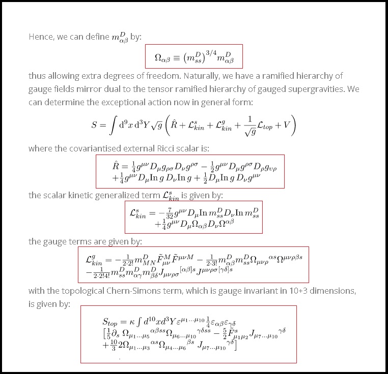
Hence, we can define $m_{\alpha \beta }^D$ by:

${\Omega _{\alpha \beta }} \equiv {\left( {m_{ss}^D} \right)^{3/4}}m_{\alpha \beta }^D$

thus allowing extra degrees of freedom. Naturally, we have a ramified hierarchy of gauge fields mirror dual to the tensor ramified hierarchy of gauged supergravities. We can determine the exceptional action now in general form:

$S = \int {{{\rm{d}}^9}} x\,{{\rm{d}}^3}Y\sqrt g \left( {\hat R + \mathcal{L}_{kin}^s + \mathcal{L}_{kin}^g + \frac{1}{{\sqrt g }}{\mathcal{L}_{top}} + V} \right)$

where the covariantised external Ricci scalar is:

$\begin{array}{l}\hat R = \frac{1}{4}{g^{\mu \nu }}{D_\mu }{g_{\rho \sigma }}{D_\nu }{g^{\rho \sigma }} - \frac{1}{2}{g^{\mu \nu }}{D_\mu }{g^{\rho \sigma }}{D_\rho }{g_{\upsilon \rho }}\\ + \frac{1}{4}{g^{\mu \nu }}{D_\mu }{\rm{In}}\,g\,{D_\nu }{\rm{In}}\,g + \frac{1}{2}{D_\mu }{\rm{In}}\,g\,{D_\nu }{g^{\mu \nu }}\end{array}$

the scalar kinetic generalized term $\mathcal{L}_{kin}^s$ is given by:

$\begin{array}{c}\mathcal{L}_{kin}^s = - \frac{7}{{32}}{g^{\mu \nu }}{D_\mu }{\rm{In}}\,m_{ss}^D{D_\nu }{\rm{In}}\,m_{ss}^D\\ + \frac{1}{4}{g^{\mu \nu }}{D_\mu }{\Omega _{\alpha \beta }}{D_\nu }{\Omega ^{\alpha \beta }}\end{array}$

the gauge terms are given by:

$\begin{array}{l}\mathcal{L}_{kin}^g = - \frac{1}{{2 \cdot 2!}}m_{MN}^D{{\tilde F}_{\mu \nu }}^M{{\tilde F}^{\mu \nu M}} - \frac{1}{{2 \cdot 3!}}m_{\alpha \beta }^Dm_{ss}^D{\Omega _{\mu \nu \rho }}^{\alpha s}{\Omega ^{\mu \nu \rho \beta s}}\\ - \frac{1}{{2 \cdot 2!4!}}m_{ss}^Dm_{\alpha \gamma }^Dm_{\beta \delta }^D{J_{\mu \nu \rho \sigma }}^{\left[ {\alpha \beta } \right]s}{J^{\mu \nu \rho \sigma }}^{\left[ {\gamma \delta } \right]s}\end{array}$

with the topological Chern-Simons term, which is gauge invariant in 10+2 dimensions, is given by:

$\begin{array}{l}{S_{top}} = \kappa \int {{d^{10}}} x{d^3}Y{\varepsilon ^{{\mu _1}...{\mu _{10}}}}\frac{1}{4}{\varepsilon _{\alpha \beta }}{\varepsilon _{\gamma \delta }}\\\left[ {\frac{1}{5}{\partial _s}} \right.{\Omega _{{\mu _1}...{\mu _5}}}^{\alpha \beta ss}{\Omega _{{\mu _6}...{\mu _{10}}}}^{\gamma \delta ss} - \frac{5}{2}{{\tilde F}_{{\mu _1}{\mu _2}}}^s{J_{{\mu _7}...{\mu _{10}}}}^{\gamma \delta }\\ + \frac{{10}}{3}2{\Omega _{{\mu _1}...{\mu _3}}}^{\alpha s}{\Omega _{{\mu _4}...{\mu _6}}}^{\beta s}\left. {{J_{{\mu _7}...{\mu _{10}}}}^{\gamma \delta }} \right]\end{array}$

and our scalar potential:

$V = \frac{1}{4}{m^{{D^{ss}}}}\left( {{\partial _s}{\Omega ^{\alpha \beta }}{\partial _s}{\Omega _{\alpha \beta }} + {\partial _s}{g^{\mu \nu }}{\partial _s}{g_{\mu \nu }} + {\partial _s}{\rm{In}}g{\partial _s}{\rm{In}}g} \right)$

$+$

$\frac{9}{{32}}{m^{{D^{ss}}}}{\partial _s}{\rm{In}}m_{ss}^D{\partial _s}{\rm{In}}m_{ss}^D - \frac{1}{2}{m^{{D^{ss}}}}{\partial _s}m_{ss}^D{\partial _s}{\rm{In}}g$

$+$

$\begin{array}{l}m{_{MN}^D^{3/4}}\left[ {\frac{1}{4}{\Omega ^{\alpha \beta }}{\partial _\alpha }{\Omega ^{\gamma \delta }}{\partial _\beta }{\Omega _{\gamma \delta }} + \frac{1}{2}{\Omega ^{\alpha \beta }}{\partial _\alpha }{\Omega ^{\gamma \delta }}{\partial _\gamma }{\Omega _{\delta \beta }}} \right.\\ + {\partial _\alpha }{\Omega ^{\alpha \beta }}{\partial _\beta }{\rm{In}}\left( {{g^{1/2}}m{{_{MN}^D}^{3/4}}} \right)\end{array}$

$+$

$\begin{array}{l}\frac{1}{4}{\Omega ^{\alpha \beta }}\left( {{\partial _\alpha }{g^{\mu \nu }}{\partial _\beta }{g_{\mu \nu }} + {\partial _\alpha }{\rm{In}}g{\partial _\beta }{\rm{In}}g} \right.\\ + \frac{1}{4}{\partial _\beta }{\rm{In}}m_{ss}^D{\partial _\beta }{\rm{In}}m_{ss}^D + \frac{1}{2}{\partial _\alpha }\left. {{\rm{In}}g{\partial _\beta }\left. {{\rm{In}}m_{ss}^D} \right)} \right]\end{array}$

and the equation of motion for the field ${J_{\mu \nu \rho }}$ is:

$\begin{array}{c}{\partial _s}\left( {\frac{\kappa }{2}{\varepsilon ^{{\mu _1}...{\mu _9}}}{\varepsilon _{\alpha \beta }}{\varepsilon _{\gamma \delta }}{\Omega _{{\mu _5}...{\mu _9}}}^{\gamma \delta ss} - } \right.\\e\frac{1}{{48}}m_{ss}^Dm_{\alpha \gamma }^D\left. {m_{\beta \delta }^D{J^{{\mu _1}...{\mu _4}\gamma \delta s}}} \right) = 0\end{array}$

U-duality entails that ${\rm{SL}}\left( 2 \right) \times {\mathbb{R}^ + }$ field theory is equivalent to 11-D and 10-D IIB supergravity under the exceptional Kaluza-Klein splitting, and the relation between M-theory and F-theory is explicitly expressed by:

$\left( {{g_{\mu \nu }},m_{MN}^D,A_\mu ^M,B_{\mu \nu }^{\alpha ,s},{C_{\mu \nu \rho }}^{\alpha \beta ,s},{D_{\mu \nu \rho \sigma }}^{\alpha \beta ,ss}} \right)$

for exceptional F-theory, and:

$\left\{ {\begin{array}{*{20}{c}}{\left( {{G_{\mu \nu }},{\gamma _{\alpha \beta }},A_\mu ^\alpha ,{{\hat C}_{\hat \mu \hat \nu \hat \rho }}} \right){\quad _{,\;}}{\rm{M - theory}}}\\{\left( {A_\mu ^M,{B_{\mu \nu }}^{\alpha ,s},{C_{\mu \nu \rho }}^{\alpha \beta ,s},{D_{\mu \nu \rho \sigma }}^{\alpha \beta ,ss}} \right){\quad _,}\;{\rm{T - IIB}}}\end{array}} \right.$

The correspondences can be written as such:

M-theory has the section condition ${\partial _s} = 0$ . The fields functionally depend on $\left( {{x^\mu },{y^\alpha }} \right)$ which are associated with the coordinates of 11-D supergravity in a 9+2 Kaluza-Klein splitting. Extra degrees of freedom come from the spacetime metric, with the Kaluza-Klein field:

${A_\mu }^\alpha = {\gamma ^{\alpha \beta }}{G_{\mu \beta }}$

and the gauge fields:

$\left( {\gamma = \det {\gamma _{\alpha \beta }}} \right)$

with:

$\left\{ {\begin{array}{*{20}{c}}{{g_{\mu \nu }} = {\gamma ^{1/7}}\left( {{G_{\mu \nu }} - {\gamma _{\alpha \beta }}{A_\mu }^\alpha {A_\nu }^\beta } \right)}\\{{\Omega _{\alpha \beta }} = {\gamma ^{ - 1/7}}{\gamma _{\alpha \beta }}}\\{m_{MN}^D = {\gamma ^{ - 6/7}}}\end{array}} \right.$

and:

$\left\{ {\begin{array}{*{20}{c}}{{A_\mu }^s = \frac{1}{2}{\varepsilon ^{\alpha \beta }}{{\hat C}_{\mu \nu \beta }}}\\{{B_{\mu \nu }}^{\alpha ,s} = {\varepsilon ^{\alpha \beta }}{{\hat C}_{\mu \nu \beta }} + \frac{1}{2}{\varepsilon ^{\beta \gamma }}{A_{\left[ {{\mu ^\alpha }{{\hat C}_\nu }} \right]\beta \gamma }}}\\{{C_{\mu \nu \rho }}^{\alpha \beta ,s} = {\varepsilon ^{\alpha \beta }}\left( {\hat C - 3{A_{\left[ {{\mu ^\gamma }{{\hat C}_{\upsilon \rho }}} \right]\gamma }} + 2{A_{{{\left[ {{\mu ^\gamma }{A_\nu }} \right]}^\delta }}}{{\hat C}_{\rho \gamma \delta }}} \right)}\end{array}} \right.$

In the IIB case, we have ${\partial _\alpha } = 0$ and the coordinate-dependence is on $\left( {{x^\mu },{y^s}} \right)$ and become the coordinates of 10-D type IIB supergravity in a 9+1 Kaluza-Klein split. The spacetime metric contribution comes from $\phi \equiv {G_{ss}}$ and the Kaluza-Klein field is hence:

${A_\mu }^s = {\phi ^{ - 1}}{G_{\mu s}}$

which parametrise the external metric and the components of the generalised metric as:

${g_{\mu \nu }} = {\phi ^{1/7}}\left( {{G_{\mu \nu }} - \phi {A_\mu }^s{A_\nu }^s} \right)$

$m_{\alpha \beta }^D = {\phi ^{ - 6/7}}{\Omega _{\alpha \beta }}$

$m_{ss}^D = {\phi ^{8/7}}$

It is clear now that the Kaluza-Klein field ${A_\mu }^s$ is identical $s$ -component-wise to the gauge field ${A_\mu }^M$ and the parametrisation of ${\Omega _{\alpha \beta }}$ in terms of the axio-dilaton

$\tau = {C_0} + i{e^{ - \varphi }}$

is given by:

${\Omega _{\alpha \beta }} = \frac{1}{{{\tau _2}}}\left( {\begin{array}{*{20}{c}}1&{{\tau _1}}\\{{\tau _1}}&{{{\left| \tau \right|}^2}}\end{array}} \right) = {e^\phi }\left( {\begin{array}{*{20}{c}}1&{{C_0}}\\{{C_0}}&{C_0^2 + {e^{ - 2\varphi }}}\end{array}} \right)$

The gauge dualities are:

${A_\mu }^\alpha = {\hat C_{\mu s}}^\alpha \,,\quad {B_{\mu \nu }}^{\alpha ,s} = {\hat C_{\mu \nu }}^\alpha + {A_{\left[ {{\mu ^s}{{\hat C}_\nu }} \right]s}}^\alpha$

$\begin{array}{l}{C_{\mu \nu \rho }}^{\alpha \beta ,s} = {\varepsilon ^{\alpha \beta }}{{\hat C}_{\mu \nu \rho s}} + 3{{\hat C}_{\left[ {\mu \left| s \right|} \right.}}\left[ {^\alpha {{\hat C}^\beta }_{\left. {\nu \rho } \right]}} \right]\\ - 2{{\hat C}_{\left[ {\mu \left| s \right|} \right.}}{\left[ {^\alpha {{\hat C}^\beta }_{\nu \left| s \right|}{A_\rho }} \right]^s}\end{array}$

$\begin{array}{l}{D_{\mu \nu \rho \sigma }}^{\alpha \beta ,s}{\varepsilon ^{\alpha \beta }}\left( {{{\hat C}_{\mu \nu \rho \sigma }} + 4{A_{\left[ {_\mu {{\hat C}_{\mu \nu \rho }}} \right]s}}} \right) + \\6{{\hat C}_{{{\left[ {{{_{\mu \nu }}^{\left[ \alpha \right.}}{{\hat C}_{\rho \left| s \right|}}^{\left. \beta \right]}{A_\sigma }} \right]}^s}}}\end{array}$

which establish not just an equivalence between ${\rm{SL}}\left( 2 \right) \times {\mathbb{R}^ + }$ -EFT and 11-D supergravity and 10-D type IIB supergravity, but also with F-theory:

which “is what results when KK-compactifying M-theory on an elliptic fibration (which yields type IIA superstring theory compactified on a circle–fiber bundle) followed by T-duality with respect to one of the two cycles of the elliptic fiber. The result is (uncompactified) type IIB superstring theory with axio-dilaton given by the moduli of the original elliptic fibration, see below. Or rather, this is type IIB string theory with some non-perturbative effects included, reducing to perturbative string theory in the Sen limit. With a full description of M-theory available also F-theory should be a full non-perturbative description of type IIB string theory, but absent that it is some kind of approximation. For instance while the modular structure group of the elliptic fibration in principle encodes (necessarily non-perturbative) S-duality effects, it is presently not actually known in full detail how this affects the full theory, notably the proper charge quantization law of the 3-form fluxes, see at S-duality – Cohomological nature of the fields under S-duality for more on that.”

Hence, in our context, F-theory is a 12-D lift of IIB supergravity yielding a geometric interpretation on the ${\rm{SL}}\left( 2 \right)$ -duality symmetry. By KK-compactifying M-theory on an elliptic fibration, we naturally have an M-theory/F-theory duality, and the ${\rm{SL}}\left( 2 \right) \times {\mathbb{R}^ + }$ -EFT although a manifest 12-D theory, however reduces to 11-D and type IIB supergravity field-theories due to topological features of worldvolumes of sevenbranes monodromy. James Halverson has an excellent exposition on that here.