On Orbifold Compactifications, D/p-Branes and Strings

By George Shiber Wednesday, April 27, 2016Saturday, August 17, 2019 In Grand Unification Physics, M Theory, Mathematical Physics, Mathematics, Philosophy Of Physics, Physics, Super String Theory compactification, mathematics

For a full mathematical definition of ‘orbifold’ summarized above, check A. Adem and M. Klaus. String-theory compactifications on N-dimensional orbifolds is attractive, and essential in some cases. For N = 6, it allows the full determination of the emergent four-dimensional effective supergravity theory, including the gauge group and matter content, the superpotential and Kähler potential, as well as the gauge kinetic function, and yields the four-dimensional space-time supersymmetry-RT.

Before proceeding, what is in an equation like …

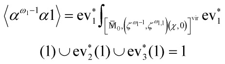
Eq. 1

where integration on a global quotient $\chi = \left[ {M/G} \right]$ is defined by

$\int_\chi \omega : = \frac{1}{{\left| G \right|}}\int_M \omega$

and $\omega \in {\Omega ^p}\left( M \right)$ is a G-invariant differential form, where $I\chi$ is the inertia stack of $\chi$ , an orbifold groupoid, yeilding the Poincaré pairing on $I\chi$ defined as the direct sum of the pairings

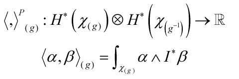
Eq. 2

with

${\rm{e}}{{\rm{v}}_i}:{\not \bar {\rm M}_{0,n}}\left( {\chi ,\beta } \right) \to I\chi$

Let us go one small mathematical step at a time, and here is a nice visualization of an orbifold

Orbi-pic

Take two D-branes, with their world-volumes and velocities ${V_1} = \tanh {v_1}$ , ${V_2} = \tanh {v_2}$ with transverse positions ${\mathord{\buildrel{\lower3pt\hbox{$\scriptscriptstyle\rightharpoonup$}} \over Y} _1}$ , ${\mathord{\buildrel{\lower3pt\hbox{$\scriptscriptstyle\rightharpoonup$}} \over Y} _2}$ . Generally, the potential between D-branes is given by cylinder vacuum amplitudes and can be interpreted as the Casimir energy stemming from open string vacuum fluctuations. The closed string amplitude

Eq. 3

is a tree level propagation between two boundary states with two sectors, RR and NSNS, corresponding to periodicity and anti-periodicity of the fermionic fields around the cylinder. Statically, we have Neumann b.c. in time and Dirichlet b.c. in space, and the dynamics of the boundary state is given by boosting the static one with a negative rapidity $v = {v_1} - {v_2}$

$\left| {B,V,{{\mathord{\buildrel{\lower3pt\hbox{$\scriptscriptstyle\rightharpoonup$}} \over Y} }_1}} \right\rangle = {e^{iv{J^{01}}}}\left| {B,\mathord{\buildrel{\lower3pt\hbox{$\scriptscriptstyle\rightharpoonup$}} \over Y} } \right\rangle$

In the large distance limit $b \to \infty$ only world-sheets with $l \to \infty$ will contribute. Hence, the moving boundary states, Eq. 4 and 5:

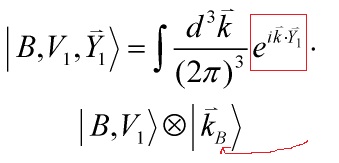
Eq. 4

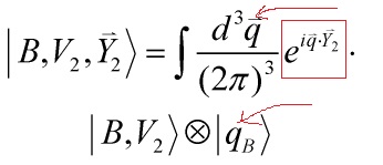
Eq. 5

can only carry space-time momentum in the combinations

$k_B^\mu = \left( {\sinh {v_1}{k^1},\cosh {v_1}{k^1},{{\mathord{\buildrel{\lower3pt\hbox{$\scriptscriptstyle\rightharpoonup$}} \over k} }_T}} \right)$

and

$q_B^\mu = \left( {\sinh {v_2}{q^1},\cosh {v_2}{q^1},{{\mathord{\buildrel{\lower3pt\hbox{$\scriptscriptstyle\rightharpoonup$}} \over q} }_T}} \right)$

If one integrates over the bosonic zero modes and factors-in momentum conservation

$\left( {k_B^\mu = q_B^\mu } \right)$

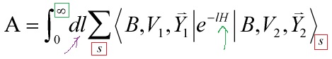
then the amplitude factorizes into a bosonic and a fermionic partition functions

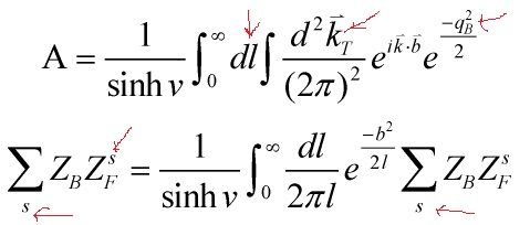
Eq. 6

where

${Z_{B,F}} = \left\langle {{B_1},{V_1}\left| {{e^{ - lH}}} \right|{B_1},{V_2}} \right\rangle _{B,F}^s$

and ${X^\mu } \equiv X_{osc}^\mu$ , and the commutation relations are

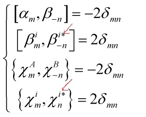
CRs

For the RR zero modes satisfying a Clifford algebraic structure and thus are proportional to $\Gamma$ -matrices

$\left\{ {\begin{array}{*{20}{c}}{\psi _0^\mu = i\,{\Gamma ^\mu }/\sqrt 2 }\\{\tilde \psi _0^\mu = i\,{{\tilde \Gamma }^\mu }/\sqrt 2 }\end{array}} \right.$

the creation annihilation operators are given by

$\left\{ {\begin{array}{*{20}{c}}{a,{a^ * } = \frac{1}{2}\left( {{\Gamma ^0} \pm {\Gamma ^1}} \right)}\\{{b^i}{b^{i * }} = \left( { - i{\mkern 1mu} {\Gamma ^i} \pm {\Gamma ^{i + 1}}} \right)}\end{array}} \right.$

thus satisfying the algebra: $\left\{ {a,{a^ * }} \right\} = \left\{ {{b^i},{b^{i * }}} \right\} = 1$

Hence, for an orbifold rotation $\left( {{g_a} = {e^{2\pi i{z_a}}}} \right)$ , we have

$\left\{ {\begin{array}{*{20}{c}}{\beta _n^a \to {g_a}\beta _n^a}\\{\beta _n^{a * } \to g_a^ * \beta _n^{a * }}\end{array}} \right.$

$\left\{ {\begin{array}{*{20}{c}}{\chi _n^a \to {g_a}\chi _n^a}\\{\chi _n^{a * } \to g_a^ * \chi _n^{a * }}\end{array}} \right.$

and

$\left\{ {\begin{array}{*{20}{c}}{{b^a} \to {g_a}{b^a}}\\{{b^{a * }} \to g_a^ * {b^{a * }}}\end{array}} \right.$

and for a boost of rapidity $v$ , we have

$\left\{ {\begin{array}{*{20}{c}}{{\alpha _n} \to {e^{ - v}}{\alpha _n}}\\{{\beta _n} \to {e^v}{\beta _n}}\end{array}} \right.$

$\left\{ {\begin{array}{*{20}{c}}{\chi _n^A \to {e^{ - v}}\chi _n^A}\\{\chi _n^B \to {e^v}\chi _n^B}\end{array}} \right.$

and

$\left\{ {\begin{array}{*{20}{c}}{a \to {e^{ - v}}a}\\{{a^ * } \to {e^v}{a^ * }}\end{array}} \right.$

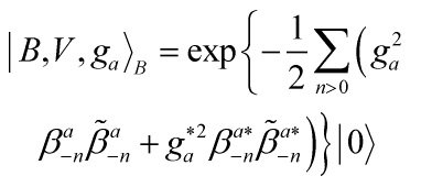
finally getting us

$\left| B \right\rangle = {\left| B \right\rangle _B} \otimes {\left| {{B_0}} \right\rangle _F} \otimes {\left| {{B_{osc}}} \right\rangle _F}$

An orbifold compactification can be obtained by identifying points in the compact part of spacetime which are connected by discrete rotations

$g = {e^{2\pi i}}\sum\limits_a {{z_a}} {J_{aa + 1}}$

on some of the compact pairs ${X^a},{\chi ^a},\quad a = 4,6,8$ and to preserve at least one supersymmetry, one imposes $\sum\limits_a {{z_a}} = 0$ .

Since 3-branes, in a double-geometric e-folding sense, figure essentially in my last few posts on the Randall-Sandrum/Klebanov-Strassler relation/correspondence, let me consider such a 3-brane configuration: in the static case, I shall take Neumann b.c. for time, Dirichlet b.c. for space and mixed b.c. for each pair of compact directions.

We get new b.c. for the compact directions

Eq. 8

Eq. 9

and

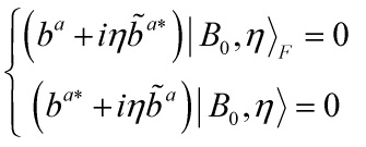
Eq. 10

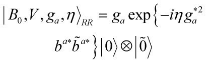
Let us also define a new spinor vacuum

$\left| {0 > \otimes \left| {\tilde 0} \right\rangle } \right.$

such that

${b^a}\left| 0 \right\rangle = {\tilde b^a}\left| {\tilde 0} \right\rangle = 0$

is the compact part of the boundary state. Notice though that

the boundary state is not invariant under orbifold rotations, under which the modes of the fields transform as in eq. (3)

Eq. 3

as well as the new spinor vacuum as

$\left| {0 > \otimes \left| {\tilde 0} \right\rangle } \right. \to {g_a}\left| 0 \right\rangle \otimes \left| {\tilde 0} \right\rangle$

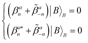
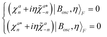
However, this was to be expected since a ${Z_N}$ rotation mixes two directions with different b.c, and hence the corresponding closed string state does not need to be invariant under ${Z_N}$ rotations. So we get for the compact part of the twisted boundary state

Eq. 11

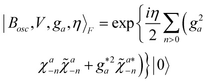
Eq. 12

and

Eq. 13

and after the GSO projection, the total partition functions for any relative angle ${w_a}$ are

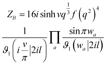
Prd. 14

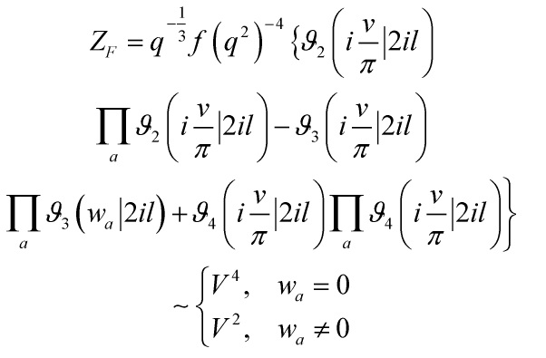
Rel. 15

and to get the invariant amplitude, one averages over all possible angles ${w_a}$ and orbifoidal-products with respect to Eq.s 1 and 2 at the beginning of this post: the mathematical beauty and the beast have became one – which at the large distance limit $l \to \infty$ , for 3-branes, but is generalizable, yields us our desired results

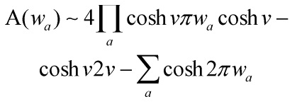
‘Eq’/~ 16

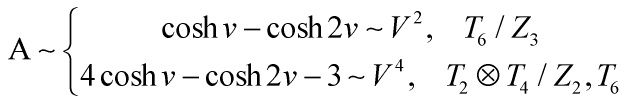
‘Eq’/~ 17

By local monodromy along the orbibold boundary circle, one gets

${\rm A} \sim \cosh v - 1 \sim {V^2}$

Thus all the D-brane configurations I have considered correspond to extremal 0-brane solutions of the low energy 4-dimensional supergravity, and the 3-brane configuration, by Eq. 1

Eq. 1

applied to the corresponding 4-D world-volume’s Kappa-terms substituted-in, gives us the Randall-Sundrum $5dB/M$ -compactification desired, visually …

nextblog1

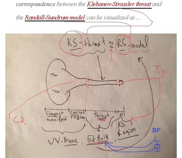
Clearly, I must cash-in on my generalization-claim above and

I plan to apply orbifold-compactification-methodology in the context of brane-cosmology, where I hope to show how it resolves the Wheeler-deWitt ‘Problem of Time’.

On Orbifold Compactifications, D/p-Branes and Strings

Thus all the D-brane configurations I have considered correspond to extremal 0-brane solutions of the low energy 4-dimensional supergravity, and the 3-brane configuration, by Eq. 1

applied to the corresponding 4-D world-volume’s Kappa-terms substituted-in, gives us the Randall-Sundrum $5dB/M$ -compactification desired, visually …

I plan to apply orbifold-compactification-methodology in the context of brane-cosmology, where I hope to show how it resolves the Wheeler-deWitt ‘Problem of Time’.

Randall-Sundrum Compactification Models and Bulk-Field Actions

Gromov – Witten Invariants, The W/K – Tau – function and Hodge Integrals

About Me

Social Networks

Archives

Login Below

Photo Gallery

Thus all the D-brane configurations I have considered correspond to extremal 0-brane solutions of the low energy 4-dimensional supergravity, and the 3-brane configuration, by Eq. 1

applied to the corresponding 4-D world-volume’s Kappa-terms substituted-in, gives us the Randall-Sundrum -compactification desired, visually …

I plan to apply orbifold-compactification-methodology in the context of brane-cosmology, where I hope to show how it resolves the Wheeler-deWitt ‘Problem of Time’.

Randall-Sundrum Compactification Models and Bulk-Field Actions

Gromov – Witten Invariants, The W/K – Tau – function and Hodge Integrals

RELATED

F-theory as the Modular Equivariant 12-D Lift of Type-IIB String Theory

Exceptional Field Theory and M-Theory on Kovalev TCS G2-Manifolds

The Wess–Zumino–Witten–Novikov Model, Taub-NUT Spaces, and M-Theory

About Me

Social Networks

Archives

Login Below

Photo Gallery

applied to the corresponding 4-D world-volume’s Kappa-terms substituted-in, gives us the Randall-Sundrum $5dB/M$ -compactification desired, visually …