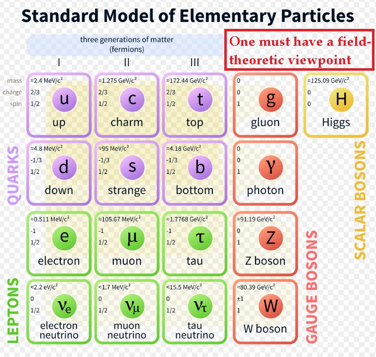
Randall-Sundrum Braneworld Scenario, Klebanov-Strassler Geometry and the Standard Model

By George Shiber Tuesday, August 1, 2017Sunday, March 31, 2019 In Cosmology, Mathematical Physics, Mathematics, Physics, Super String Theory Klebanov-Strassler Geometry, Randall–Sundrum model

In this post, the mathematics applies to both, Randall-Sundrum-1and-2 models, hence I will not distinguish between them here. One of the most powerful aspects of M-theory’s braneworld scenarios is that the bosonic and fermionic fields of the Standard Model of physics can be interpreted as low-lying Kaluza-Klein excitations of Randall-Sundrum bulk fields, after extra dimensional modulus stabilization, and recalling that Randall-Sundrum bulk/brane interactions yield a very deep solution to the EW hierarchy problem. Start with the theory defined by the following action:

$S = \frac{1}{2}\int {{d^4}} x\int\limits_{ - \pi }^\pi {d\phi \sqrt G } \left( {{G^{AB}}{\partial _A}\Phi {\partial _B}\Phi - {m^2}{\phi ^2}} \right)$

with the bulk field given by:

$\Phi \left( {x,\phi } \right) = \sum\limits_n {\frac{{{\Upsilon _n}\left( \phi \right)}}{{\sqrt {{\tau _c}} }}}$

where generally, the bulk action, with worldsheet-uplift, is given by:

$\begin{array}{l}{S_B} = - \frac{1}{{2{k^2}}}\int {{d^D}} X\left\{ {\frac{1}{2}} \right.\left[ {{\eta ^{\mu \rho }}} \right.{\eta ^{\nu \sigma }} + {\eta ^{\mu \sigma }}{\eta ^{\nu \rho }}\\ - \frac{2}{{D - 2}}{\eta ^{\mu \nu }}\left. {{\eta ^{\rho \sigma }}} \right]{h_{\mu \nu }}{\partial ^2}{h_{\rho \sigma }}\left. { + \frac{4}{{D - 2}}\bar \Phi {\partial ^2}\bar \Phi } \right\}\end{array}$

and ${\Upsilon _n}\left( \phi \right)$ satisfying:

$\int\limits_{ - \pi }^\pi {d\phi {e^{ - \sigma \left( \phi \right)}}} {\Upsilon _n}\left( \phi \right){\Upsilon _m}\left( \phi \right) = {\delta _{nm}}$

with a Dirac-Born-Infeld brane interaction term:

${S_{BI}} = - {\tau _\rho }\int {{d^{p + 1}}} \xi \left( {\left( {\frac{{2p - D + 4}}{{D - 2}}} \right)\bar \Phi - \frac{1}{2}{h_{aa}}} \right)$

which, after integration by parts and upon substituting ${e^{ - \sigma \left( \phi \right)}}$ in our action, we get the Horava-Witten action variant:

$\begin{array}{c}S = \frac{1}{2}\int {{d^4}} x\int\limits_{ - \pi }^\pi {{r_c}d\phi } \left( {{e^{ - 2\sigma \left( \phi \right)}}} \right.\\{\eta _{\mu \nu }}{\partial _\mu }\Phi {\partial _\nu }\Phi + \frac{1}{{r_c^2}}\left( {{e^{ - 4\sigma \left( \phi \right)}}\partial \Phi } \right)\\ - {m^2}{e^{ - 4\sigma \left( \phi \right)}}\left. {{\Phi ^2}} \right)\end{array}$

Now, the bulk fields manifest themselves to 4-D ‘observers’ as infinite towers of scalars ${\psi _n}\left( x \right)$ with masses ${m_n}$ . After change of variables to:

$\left\{ {\begin{array}{*{20}{c}}{{z_n} = {m_n}{e^{\sigma \left( \phi \right)}}/k}\\{{f_n} = {e^{ - 2\sigma \left( \phi \right)}}{\Upsilon _n}}\end{array}} \right.$

our actions reduce to two interaction terms:

$S_{{\mathop{\rm int}} }^G = \int {{d^4}} x\int\limits_{ - \pi }^\pi {d\phi \sqrt G } \frac{\lambda }{{{M^{5m - 5}}}}{\left( {{G^{AB}}{\partial _A}\Phi {\partial _B}\Phi } \right)^m}$

and:

$\begin{array}{l}S_{{\mathop{\rm int}} }^\Upsilon = \int {{d^4}} x\int\limits_{ - \pi }^\pi {{r_c}} d\phi {e^{ - 4\sigma \left( \phi \right)}}\frac{\lambda }{{{M^{5m - 5}}}} \cdot \\\psi _n^{2m}\left( {\frac{{{{\left( {{\partial _\phi }{\Upsilon _n}} \right)}^2}}}{{r_c^3}}} \right)\end{array}$

where we have:

$z_n^2\frac{{{d^2}{f_n}}}{{dz_n^2}} + {z_n}\frac{{d{f_n}}}{{d{z_n}}} + \left[ {z_n^2 - \left( {4 + \frac{{{m^2}}}{{{k^2}}}} \right)} \right]{f_n} = 0$

and the Bessel functions of order:

$v = \sqrt {4 + \frac{{{m^2}}}{{{k^2}}}}$

yield the standard Bertotti-Robinson-solutions. Hence, we have:

$\begin{array}{*{20}{l}}{{\Upsilon _n}\left( \phi \right) = \frac{{{e^{2\sigma \left( \phi \right)}}\phi }}{{{N_n}}}\left[ {{J_\nu }\left( {\frac{{{m_n}}}{k}{e^{\sigma \left( \phi \right)}}} \right)} \right. + }\\{\left. {{b_{n\nu }}{\Upsilon _\nu }\left( {\frac{{{m_n}}}{k}{e^{\sigma \left( \phi \right)}}} \right)} \right]}\end{array}$

with ${N_n}$ a normalization factor. That the differential operator on the LHS of:

$- \frac{1}{{r_c^2}}\frac{d}{{d\phi }}\left( {{e^{ - 4\sigma \left( \phi \right)}}\frac{{d{\Upsilon _n}}}{{d\phi }}} \right) + {m^2}{e^{ - 4\sigma \left( \phi \right)}}{\Upsilon _n} = m_n^2{e^{ - 2\sigma \left( \phi \right)}}{\Upsilon _n}$

is self-adjoint means that the derivative of ${y_n}\left( \phi \right)$ is continuous at the orbifold fixed points, giving us:

$\left\{ {\begin{array}{*{20}{c}}{{N_n} \simeq \frac{{{e^{k{r_c}\pi }}}}{{\sqrt {k{r_c}} }}{A_n}}\\{{A_n} = {J_n}\left( {{x_{n\nu }}} \right)\sqrt {1 + \frac{{4 - {\nu ^2}}}{{x_{n\nu }^2}}} }\end{array}} \right.$

Four-dimensionally, these induce couplings between the Kaluza-Klein modes and so the exponential factor in:

$\left\{ {\begin{array}{*{20}{c}}{d{s^2} = {e^{ - 2k{r_c}\left| \phi \right|}}{\eta _{\eta \nu }}}\\{d{x^\mu }d{x^\nu } - r_c^2d{\phi ^2}}\end{array}} \right.$

where ${x^\mu }$ are Lorentz coordinates on the four-dimensional surfaces of constant $\phi$ thus plays an essential role in determining the effective scale of the couplings. If the Planck scale sets the scale of the five-dimensional couplings, the low-lying Kaluza-Klein modes will have TeV-range self-interactions.

Now, a Klebanov-Strassler geometry naturally arises by considering string theory compactification on $Ad{S_5} \times {X_5}$ where ${X_5}$ is the Einstein manifold in five dimensions, with the interaction-Lagrangian of the massless Klebanov-Strassler field and the brane fields fermions is:

$\begin{array}{*{20}{c}}{{\mathcal{L}^{KS}}_{\psi \bar \psi {H^0}}\frac{1}{{{M^{3/2}}}}\bar \psi \left[ {i{\gamma ^\mu }} \right.{\sigma ^{\mu \nu }}H_{\mu \nu \lambda }^0\left( {{x^\mu }} \right)}\\{\left. {\frac{{{\chi ^0}(r)}}{{\sqrt {\tau c} }}} \right]\psi }\end{array}$

which, after integrating over the extra dimensional part, the effective 4-D Lagrangian reduces to:

$\begin{array}{*{20}{c}}{\mathcal{L}_{\psi \bar \psi {H^0}}^{KS} = i\bar \psi {\gamma ^\mu }{\sigma ^{\mu \nu }}\left[ {\frac{{{e^{ - 4\pi K/{3_{{g_s}}}M}}}}{{{M_{pl}}}}} \right. \cdot }\\{\left. {\left( {\frac{{{r_{\max }}}}{{{r_0}}}} \right)} \right]H_{\mu \nu \lambda }^0\psi }\end{array}$

with the fundamental Planck scale $M$ and the 4-D Planck scale ${M_{pl}}$ related as

${M_{pl}} = \frac{{{M^{3/2}}}}{{\sqrt {2R} }}{r_{\max }}{\left( {1 - \frac{{r_0^2}}{{r_{\max }^2}}} \right)^{1/2}}$

Hence, in light of the Klebanov-Strassler/Randall-Sundrum throat-bulk isomorphism, this defines a background geometry given by:

$S = - {M^3}\int {{d^5}} x\sqrt G \left[ {R - \Lambda } \right]$

$+$

$\int {{d^5}} x\sqrt G \left[ {\frac{1}{2}{G^{MN}}{\partial _M}\Phi {\partial _N}\Phi - V\left( \Phi \right)} \right]$

$-$

$\int {{d^4}} x\sqrt { - {g_{hid}}} {\lambda _{hid}}\left( \Phi \right)$

$-$

$\int {{d^4}} x\sqrt { - {g_{vis}}} {\lambda _{vis}}\left( \Phi \right)$

with ${{g_{hid}}}$ and ${{g_{vis}}}$ the induced metric on the hidden and visible brane-sectors, ${G_{MN}}$ the 5-D metric, with $M$ the 5-D Planck scale, $\Lambda$ the cosmological ‘constant’, $\Phi$ the scalar field and ${V\left( \Phi \right)}$ the corresponding potential.

Working in the $A\left( \Phi \right)$ -warp-factor metric:

$d{s^2} = \exp \left[ { - 2A\left( \phi \right)} \right]{\eta _{\mu \nu }}d{x^\mu }d{x^\nu } - r_c^2d{\phi ^2}$

the corresponding 5-D Einstein and scalar field equations are:

$\begin{array}{l}\frac{4}{{r_c^2}}{{A'}^2}\left( \phi \right) - \frac{1}{{r_c^2}}A''\left( \phi \right) = - \frac{{2{k^2}}}{3}V\left( \Phi \right)\\ - \frac{{{k^2}}}{3}\sum {{\lambda _i}} \left( \Phi \right)\delta \left( {\phi - {\phi _i}} \right)\end{array}$

$\frac{1}{{r_c^2}}{{A'}^2}\left( \phi \right) = \frac{{{k^2}}}{{12r_c^2}}{{\Phi '}^2} - \frac{{{k^2}}}{6}V\left( \Phi \right)$

and

$\frac{1}{{r_c^2}}\Phi ''\left( \phi \right) = \frac{4}{{r_c^2}}A'\Phi ' + \frac{{\partial V}}{{\partial \Phi }} + \sum {\frac{{\partial {\lambda _i}}}{{\partial \Phi }}} \delta \left( {\phi - {\phi _i}} \right)$

with the index over the branes and our boundary-conditions of $A\left( \phi \right)$ and $\Phi \left( \phi \right)$ are given by:

$\frac{1}{{{r_c}}}{\left[ {A'\left( \phi \right)} \right]_i} = \frac{{{k^2}}}{3}{\lambda _i}\left( {{\Phi _i}} \right)$

$\frac{1}{{{r_c}}}{\left[ {\Phi '\left( \phi \right)} \right]_i} = {\partial _\Phi }{\lambda _i}\left( {{\Phi _i}} \right)$

To analytically solve in the backreacted Randall-Sundrum model-type, we use the quadratic/quartic bulk/brane dualized potential:

$V\left( \Phi \right) = \frac{1}{2}{\Phi ^2}\left( {{\upsilon ^2} + 4\upsilon k} \right) - \frac{{{k^2}}}{6}{\upsilon ^2}{\Phi ^4}$

with:

$k = \sqrt { - {k^2}\frac{\Lambda }{6}}$

Now we can derive solutions:

$A\left( \phi \right) = k{r_c}\left| \phi \right| + \frac{{{k^2}}}{{12}}\Phi _P^2{e^{ - 2\upsilon {r_c}\left| \phi \right|}}$

$\Phi \left( \phi \right) = {\Phi _P}{e^{ - \upsilon \pi {r_c}}}$

where ${\Phi _P}$ is the scalar field on the Planck brane. Hence, ${\lambda _{hid}}$ and ${\lambda _{vis}}$ are given by:

${\lambda _{hid}} = \frac{{6k}}{{{k^2}}} - \upsilon \Phi _P^2$

and

${\lambda _{vis}} - = \frac{{6k}}{{{k^2}}} - \upsilon \Phi _P^2{e^{ - 2\upsilon \pi {r_c}}}$

We can now address the modulus stability of the braneworld. Substituting ${\Phi _P}$ into:

$S = - {M^3}\int {{d^5}} x\sqrt G \left[ {R - \Lambda } \right]$

$+$

$\int {{d^5}} x\sqrt G \left[ {\frac{1}{2}{G^{MN}}{\partial _M}\Phi {\partial _N}\Phi - V\left( \Phi \right)} \right]$

$-$

$\int {{d^4}} x\sqrt { - {g_{hid}}} {\lambda _{hid}}\left( \Phi \right)$

$-$

$\int {{d^4}} x\sqrt { - {g_{vis}}} {\lambda _{vis}}\left( \Phi \right)$

gives us the 4-D potential for the radion:

${V_{eff}}\left( {{r_c}} \right) = {r_c}\int {d\phi } \exp \left[ { - 4A\left( \phi \right)} \right]\left[ {{\upsilon ^2}\Phi _P^2{e^{ - 2\upsilon {r_c}\phi }}} \right.$

$+$

$\left( {{\upsilon ^2} + 4\upsilon k} \right)\Phi _P^2\exp \left( { - 2\upsilon r{\phi _c}} \right) - \frac{{{k^2}{\upsilon ^2}}}{3}\left. {\Phi _P^4} \right]$

$\cdot$

${e^{ - 4\upsilon {r_c}\phi }} + {e^{\left[ { - 4A\left( 0 \right)} \right]\upsilon \Phi _P^2}}$

$-$

${e^{\left[ { - 4A\left( {\pi {r_c}} \right)} \right]\upsilon \Phi _P^2}}{e^{\left( {\pi - 2\upsilon \pi {r_c}} \right)}}$

One then achieves inter-brane stabilization by minimizing the above potential with respect to the radion:

$\begin{array}{l}\frac{{\partial {V_{eff}}}}{{\partial \left( {\pi {r_c}} \right)}} = {e^{\left[ { - 4A\left( {\pi {r_c}} \right)} \right]}}{e^{\left( { - 2\upsilon \pi {r_c}} \right)}} \cdot \\\left[ {4{\upsilon ^2}\Phi _P^2 + 8\upsilon k\Phi _P^2 - {k^2}{\upsilon ^2}} \right.\left. {{e^{\left( { - 2\upsilon \pi {r_c}} \right)}}} \right]\end{array}$

Hence, for the modulus field ${r_c}$ , the stabilization condition is:

$k\pi {r_c} = \frac{{4{k^2}}}{{m_\Phi ^2}}{\rm{In}}\left\{ {\frac{{{k^{{\Phi _P}}}}}{{2\sqrt {1 + \frac{{2k}}{\upsilon }} }}} \right\}$

Note now, in a backreacted RS model,

${V_{eff}}$

has no minima that is consistent with inflationary coupling-running. Thus, a quartic term of the bulk stabilising field potential must be coupled to the action factoring the mass of the scalar field:

$m_\Phi ^2 = 4\upsilon k$

Consider brane-fluctuations localized at stable inter-brane separation ${r_c}$ as a function of brane-coordinates. The metric is hence:

$d{s^2} = {e^{\left[ { - 2A\left( {x,\phi } \right)} \right]}}{g_{\mu \nu }}\left( x \right)d{x^\mu }d{x^\nu } - {T^2}\left( x \right)d{\phi ^2}$

The KK-modified brane warping is given by:

$A\left( {x,\phi } \right) = k\left| \phi \right|T\left( x \right) + \frac{{{k^2}\Phi _P^2}}{{12}}{e^{ - 2\upsilon \left| \phi \right|T\left( x \right)}}$

for $\phi$ the 5-D modulus brane angular coordinates. The Einstein-Hilbert action now is given by:

$\begin{array}{l}S_{EH}^{kin}\left[ T \right] = 12{M^3}\int {{d^4}} x\sqrt { - g} \int {d\phi {e^{ - 2A\left( {x,\phi } \right)}}} \cdot \\\left[ {k\phi {\partial _\mu }T} \right.{\partial ^\mu }T\left( {1 - \frac{{{k^2}\Phi _P^2}}{6}\frac{\upsilon }{k}{e^{ - 2A\left( {x,\phi } \right)}}} \right) - \\{k^2}{\phi ^2}T{\partial _\mu }T{\partial ^\mu }T\left. {{{\left( {1 - \frac{{{k^2}\Phi _P^2}}{6}\frac{\upsilon }{k}{e^{ - 2A\left( {x,\phi } \right)}}} \right)}^2}} \right]\end{array}$

and by integrating over the 5th dimensional scalar field, we get

$S_{EH}^\phi \left[ T \right] = \frac{{6{M^3}}}{k}\int {{d^4}} x\sqrt { - g} {\partial _\mu }{e^{ - A\left( {\pi ,x} \right)}}{\partial ^\mu }{e^{ - A\left( {\pi ,x} \right)}}$

with kinetic sub-part:

$S_{kin}^\Psi = \frac{1}{2}\int {{d^4}} x\sqrt { - g} {\partial _\mu }\Psi {\partial ^\mu }\Psi$

where $\Psi$ is the normalised radion field:

$\Psi \left( x \right) = \sqrt {\frac{{12{M^3}}}{k}} {e^{ - A\left( {x,\pi } \right)}}$

Thus, coupling the mass to the effective potential term and the inter brane measure $T\left( x \right)$ gives us:

${{V''}_{eff}}\left( {{r_c}} \right) = 2{k^2}{\upsilon ^3}{e^{ - 4A\left( {\pi {r_c}} \right)}}{e^{ - 4\upsilon \pi {r_c}}}$

and:

$T'{\left( \Psi \right)^2}\left| {_{{r_c}}} \right. = \frac{1}{{12{M^3}k}}{e^{2A\left( {\pi {r_c}} \right)}}$

hence yielding the mass term:

$\left\{ {\begin{array}{*{20}{c}}{m_\Psi ^2 = \frac{{4{k^2}\Phi _P^2}}{{3{M^3}}}{\varepsilon ^2}{e^{ - 2k\pi {r_c}}}}\\{\varepsilon = \frac{{m_\Phi ^2}}{{4{k^2}}}}\end{array}} \right.$

Standard Model physics naturally arises now. One first derives the scalar radion field via interaction terms in the Standard Model, since the metric:

$d{s^2} = {e^{\left[ { - 2A\left( {x,\phi } \right)} \right]}}{g_{\mu \nu }}\left( x \right)d{x^\mu }d{x^\nu } - {T^2}\left( x \right)d{\phi ^2}$

implies that the visible RS brane:

${\left( {\frac{\Psi }{f}} \right)^2}{g_{\mu \nu }}$

and:

$\Psi \left( x \right)$

couple to the Higgs sector of the SM via the action:

$\begin{array}{l}{S_H} = \frac{1}{2}\int {{d^4}} x\sqrt { - g} {\left( {\frac{\Psi }{f}} \right)^4}.\\\left[ {{{\left( {\frac{\Psi }{f}} \right)}^{ - 2}}{g^{\mu \nu }}{\partial _\mu }h{\partial _\nu }h - \mu _0^2{h^2}} \right]\end{array}$

$\begin{array}{l}{S_H} = \frac{1}{2}\int {{d^4}} x\sqrt { - g} {\left( {\frac{\Psi }{f}} \right)^4}.\\\left[ {{{\left( {\frac{\Psi }{f}} \right)}^{ - 2}}{g^{\mu \nu }}{\partial _\mu }H{\partial _\nu }H - \mu _0^2{H^2}} \right]\end{array}$

where $H$ is the Higgs field. Normalizing via:

$H\left( x \right) \to \frac{{\left\langle \Psi \right\rangle }}{f}H\left( x \right) \equiv \tilde H\left( x \right)$

thus reduces our action to:

$\begin{array}{l}{S_{\tilde H}} = \frac{1}{2}\int {{d^4}} x\sqrt { - g} {\left[ {\left( {\frac{\Psi }{{\left\langle \Psi \right\rangle }}} \right)} \right.^2}{g^{\mu \nu }}{\partial _\mu }H{\partial _\nu }H\\ - {\left( {\frac{\Psi }{{\left\langle \Psi \right\rangle }}} \right)^4}\left. {{\mu ^2}{H^2}} \right]\end{array}$

where:

$\mu = {\mu _0}{e^{ - A\left( {\pi {r_c}} \right)}}$

By an Euler-Lagrange derivation, we get the Higgs-field energy-momentum tensor:

$\mathcal{L} = \frac{{\delta \Psi }}{\Psi }T_\mu ^\mu H$

thus coupling the radion to the Higgs via:

${\lambda _{H - \delta H}} = \frac{{{\mu ^2}}}{{\left\langle \Psi \right\rangle }}$

It is straightforward now to generalize to all fields of the Standard Model. Let $\Xi$ be any field

By the above Higgs method, the corresponding RS-SM coupling term is:

${\lambda _{\Xi - \delta \Psi }} = \frac{{m_\Xi ^2}}{{\left\langle \Psi \right\rangle }}$

Hence, yielding the coupled action:

$\begin{array}{*{20}{l}}{{S_{\tilde H}} = \frac{1}{2}\int {{d^4}} x\sqrt { - g} {{\left[ {\left( {\frac{\Psi }{{\left\langle \Psi \right\rangle }}} \right)} \right.}^2}{g^{\mu \nu }}{\partial _\mu }\Xi {\partial _\nu }\Xi }\\{ - {{\left( {\frac{\Psi }{{\left\langle \Psi \right\rangle }}} \right)}^4}\left. {{\mu ^2}{\Xi ^2}} \right]}\end{array}$

Going back to the Klebanov-Strassler/Randall-Sundrum throat-bulk isomorphism, a stack of N D3-branes placed at the singularity ${z_i} = 0$ backreacts on the KS-geometry, creating a warped background with the following ten dimensional line element

$\begin{array}{c}d{s^2} = {h^{1/2}}(z){g_{\mu \nu }}d{x^\mu }d{x^\nu } + \\{h^{ - 1/2}}(z){g_{i\overline j }}d{z^i}d{z^{\overline j }}\end{array}$

with ${g_{i\overline j }}$ the metric

$\begin{array}{c}ds_{{T^{1,1}}}^2 = \frac{1}{6}\left( {d\psi + \sum\limits_{i = 1}^2 {\cos {\theta _i}d{\phi _i}} } \right) + \\\frac{1}{6}\sum\limits_{i = 1}^2 {\left( {d\phi _i^2 + {{\sin }^2}{\theta _i}d\phi _i^2} \right)} \end{array}$

and the warp factor is

$\left\{ {\begin{array}{*{20}{c}}{h(r) = \frac{{{R^4}}}{{{r^4}}}}\\{{R^4} \equiv \frac{{2z\pi }}{4}{g_s}N{{(\alpha ')}^2}}\end{array}} \right.$

and

the deep part is that this AdS background is an explicit realization of the Randall-Sundrum scenario in string theory

that I discussed here and here. So in line with the AdS/CFT duality, the $Ad{S_5} \times {T^{1,1}}$ geometry

has a dual gauge theory interpretation

namely, an $SU(N) \times SU(N)$ gauge theory coupled to bifundamental chiral superfields, and adding $M$ D5-branes wrapped over the ${S^2}$ inside ${T^{1,1}}$ , then the gauge group becomes

$SU\left( {N + M} \right){\rm{ }} \times {\rm{ }}SU\left( N \right)$

giving a cascading gauge theory. The three-form flux induced by the wrapped D5-branes – fractional D3-branes – satisfies

$\frac{1}{{{{\left( {2\pi } \right)}^2}\alpha '}}\int_{{S^3}} {{F_3}} = M$

and the Klebanov-Strassler warp-throat factor is

$\begin{array}{c}h(r) = \frac{{27\pi {{\left( {\alpha '} \right)}^2}}}{{4{r^2}}}\left[ {{g_s}} \right.N + \frac{2}{{2\pi }}\\{\left( {{g_s}M} \right)^2}{\rm{In}}\left( {\frac{r}{{{r_0}}}} \right) + \frac{3}{{8\pi }}\left. {{{\left( {{g_s}M} \right)}^2}} \right]\end{array}$

with

${r_0} \sim {\varepsilon ^{2/3}}{e^{2\pi N/\left( {3{g_s}M} \right)}}$

Thus from:

$\mathcal{L} = \frac{{\delta \Psi }}{\Psi }T_\mu ^\mu \Xi$

one derives the wave-function and the superposition-principle for every SM field from Kirchhoff ’s integral theorem. That gets very philosophically deep in the context of the Wheeler–DeWitt equation and the Hartle–Hawking wave function ${\Theta _{HH}}$ , since as one might expect, boundary conditions and the potential condition corresponding to the path-integral of:

$\begin{array}{*{20}{l}}{{S_{\tilde H}} = \frac{1}{2}\int {{d^4}} x\sqrt { - g} {{\left[ {\left( {\frac{{{\Theta _{HH}}}}{{\left\langle {{\Theta _{HH}}} \right\rangle }}} \right)} \right.}^2}{g^{\mu \nu }}{\partial _\mu }\Xi {\partial _\nu }\Xi }\\{ - {{\left( {\frac{{{\Theta _{HH}}}}{{\left\langle {{\Theta _{HH}}} \right\rangle }}} \right)}^4}\left. {{\mu ^2}{\Xi ^2}\mathord{\buildrel{\lower3pt\hbox{$\scriptscriptstyle\leftrightarrow$}} \over \partial } H} \right]}\end{array}$

are highly problematic, to say the least, though in upcoming posts, I will show how M-theory successfully deals with both via geometric surgery/quantum engineering methods in homological mirror symmetry.