Randall-Sundrum Cosmology and Dp-Brane Dynamics

By George Shiber Saturday, June 24, 2017Friday, October 26, 2018 In Cosmology, Dp-Branes, Mathematical Physics, Mathematics, Physics D-Branes, Randall-Sundrum Cosmology

Let me work in the large-warped Randall-Sundrum D-brane scenario and consider how an ${S^1}/{Z_2}$ orbifolding leads to a non-singular cosmic bounce on the brane thus alleviating the rip of the big-bang singularity. The Randall-Sundrum 5-D braneworld action is:

$\begin{array}{*{20}{c}}{S = \int {{d^5}} x\sqrt { - {g_{\left( 5 \right)}}} \left[ {{M^3}{R_{\left( 5 \right)}} - \Lambda } \right]}\\{ + \int {{d^4}x} \sqrt { - {g_{\left( 4 \right)}}} {\rm{ \tilde L}}_{Brane}^{{\rm{large}}}}\end{array}$

$M$ the 5-D Planck mass, ${M^3} = 1/\left( {16\pi {G_5}} \right)$ , and $\Lambda$ the cosmological constant in the bulk, yielding the metric on the brane:

$\begin{array}{c}d{s^2} = {e^{ - 2\left| y \right|/L}}\left[ {{\eta _{\mu \nu }} + {h_{\mu \nu }}\left( {x,y} \right)} \right] \cdot \\d{x^\mu }d{x^\nu } + d{y^2}\end{array}$

with $L$ being the radius of AdS, defined by:

$R_{MNPQ}^{\left( 5 \right)} = - \frac{1}{{{L^2}}}\left( {g_{MP}^{\left( 5 \right)}g_{NQ}^{\left( 5 \right)} - g_{MQ}^{\left( 5 \right)}g_{NP}^{\left( 5 \right)}} \right)$

thus allowing us to derive the CFT-brane relation:

$\begin{array}{l}{h_{\mu \nu }}\left( p \right) = - \frac{2}{{L{M^3}}}{\Delta _3}\left[ {{T_{\mu \nu }}\left( p \right) - \frac{1}{2}{\eta _{\mu \nu }}{T^\alpha }_\alpha \left( p \right)} \right]\\ - \frac{1}{{{M^3}}}{\Delta _{KK}}\left( p \right)\left[ {{T_{\mu \nu }}\left( p \right) - \frac{1}{3}{\eta _{\mu \nu }}{T^\alpha }_\alpha \left( p \right)} \right]\end{array}$

where the dynamics of N-parallel topologically intersecting Dp-branes with gauge group $U\left( N \right)$ is:

$\begin{array}{l}S = - \frac{{{T_p}{g_s}{{\left( {2\pi \alpha '} \right)}^2}}}{4}\int {{{\rm{d}}^{p + 1}}} \xi {\rm{tr}}\left( {{F_{ab}}{F^{ab}} + } \right.\\2{D_a}{\Phi ^m}{D^a}{\Phi _m} + \sum\limits_{m \ne n} {{{\left[ {{\Phi ^m},{\Phi ^n}} \right]}^2} + \left. {{\rm{fermions}}} \right)} \end{array}$

with the Yang-Mills potential being:

$V\left( \Phi \right) = {\sum\limits_{m \ne n} {\left[ {{\Phi ^m},{\Phi ^n}} \right]} ^2}$

and we have:

${F_{ab}} = {D_a}{\Phi ^m} = {\psi ^\alpha } = 0$

$V\left( \Phi \right) = 0$

The Einstein field equations in the RS theory are derived for both, the 2-stack 3-branes as well as inter-brane separation. Our 5-D ADS spacetime geometry is an

${S^1}/{Z_2}$

orbifolding and our branes are localized at orbifolded fixed points:

$\left\{ {\begin{array}{*{20}{c}}{\varphi = 0}\\{\varphi = \pi }\end{array}} \right.$

with $\varphi$ the Planck brane. The action is hence given by:

$\begin{array}{l}S = \frac{1}{{2{\kappa ^2}}}\int {{d^4}} xd\varphi \sqrt { - G} \left[ {{R^{\left( 5 \right)}} + \left( {12/{l^2}} \right)} \right]\\ - \int {{d^4}} x\left[ {\sqrt { - {g_{hid}}} {V_{hid}} + \sqrt { - {g_{vis}}} {V_{vis}}} \right]\end{array}$

with the metric being:

$d{s^2} = {\tilde b^2}\left( x \right)d{\varphi ^2} + {e^{ - 2A\left( {\varphi ,x} \right)}}{h_{\mu \nu }}\left( x \right)d{x^\mu }d{x^\nu }$

with

$A\left( {\varphi ,x} \right)$

the spacetime warped brane factor along the extra dimensions. From this, one gets the Einstein field equations as:

$\begin{array}{l}\frac{{{e^{ - 2\xi }}}}{{\tilde b}}{\left( {K_\nu ^\mu } \right)_{,\varphi }} - {e^{ - 2\xi }}KK_\nu ^\mu + R_\nu ^{\left( 4 \right)}\left( h \right)\\ - {\nabla ^\mu }{\nabla _\nu }\xi - {\nabla ^\mu }\xi {\nabla _\nu }\xi = - \frac{4}{{{l^2}}}\delta _\nu ^\mu + {\kappa ^2}\left( {\frac{1}{3}\delta _\nu ^\mu {V_{hid}}} \right)\frac{{{e^{ - \xi }}}}{{\tilde b}}\delta \left( \varphi \right)\\ + {\kappa ^2}\left( {\frac{1}{3}\delta _\nu ^\mu {V_{vis}}} \right)\frac{{{e^{ - \xi }}}}{{\tilde b}}\delta \left( {\varphi - \pi } \right)\end{array}$

$\begin{array}{l}\frac{{{e^{ - 2\xi }}}}{{\tilde b}}{K_{,\varphi }} - {e^{ - 2\xi }}{K^{\mu \nu }}{K_{\mu \nu }} - {\nabla ^\mu }{\nabla _\mu }\xi - {\nabla ^\mu }\xi {\nabla _\mu }\xi \\ = - \frac{4}{{{l^2}}} + \frac{{4{\kappa ^2}}}{3}{V_{hid}}\frac{{{e^{ - \xi }}}}{{\tilde b}}\delta \left( \varphi \right)\\ - \frac{{4{\kappa ^2}}}{3}{V_{vis}}\frac{{{e^{ - \xi }}}}{{\tilde b}}\delta \left( {\varphi - \pi } \right)\end{array}$

with the constraint:

${\nabla _\nu }\left( {{e^{ - \xi }}K_\nu ^\mu } \right) - {\nabla _\mu }\left( {{e^{ - \xi }}K} \right) = 0$

We also impose the condition that the brane curvature radius $L$ is much larger than the bulk curvature $l$ :

$\varepsilon = {\left( {\frac{l}{L}} \right)^2} \ll 1$

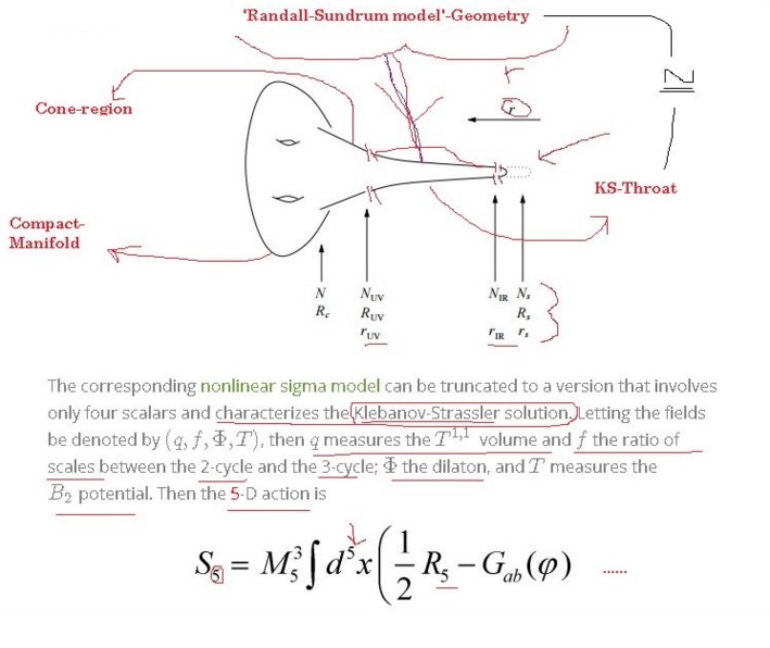
Visually, we get the following model:

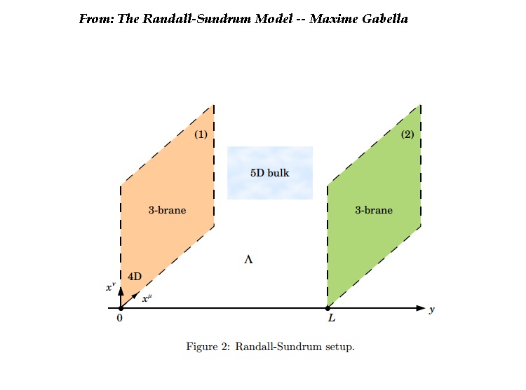
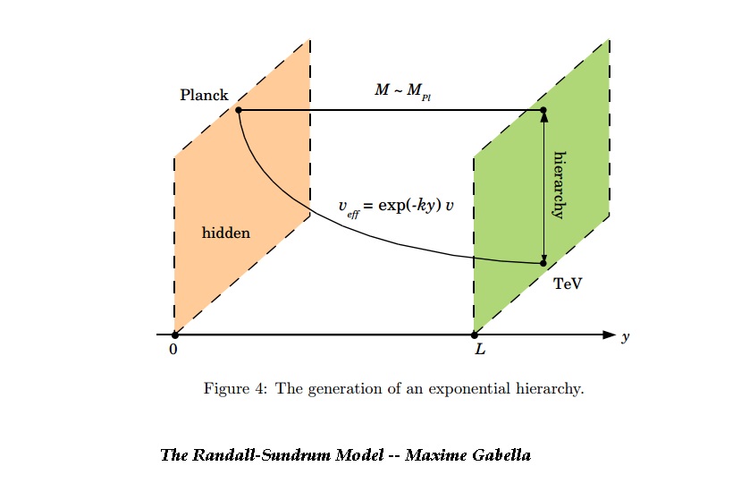
First, let us recall the remarkable way in which the Randall-Sundrum scenario solves the hierarchy problem. I will make it easy by simply quoting Graham D. Kribs:

Randall and Sundrum (RS) proposed a fascinating solution to the hierarchy problem. The setup involves two 4D surfaces (“branes”) bounding a slice of 5D compact AdS space taken to be on an S1/Z2 orbifold. Gravity is effectively localized one brane, while the Standard Model (SM) fields are assumed to be localized on the other. The wavefunction overlap of the graviton with the SM brane is exponentially suppressed, causing the masses of all fields localized on the SM brane to be exponentially rescaled. The hierarchy problem can be solved by assuming all fields initially have masses near the 4D Planck scale, and arranging that the exponential suppression rescales the Planck mass to a TeV on the SM brane. This requires stabilizing the size of the extra dimension to be about thirty-five times larger than the AdS radius. Goldberger and Wise proposed adding a massive bulk scalar field with suitable brane potentials causing it to acquire a vev with a nontrivial x5-dependent profile. The desired exponential suppression could be obtained without any large fine-tuning of parameters. Fluctuations about the stabilized RS model include both tensor and scalar modes

Now, integrating over the dimensions yields the effective 4-D action:

$\begin{array}{l}{S_{eff}} = \frac{l}{{2{\kappa ^2}}}\int {{d^4}} x\sqrt { - f} \left[ {\Phi \left( x \right)} \right.{R^{\left( 4 \right)}}\left( f \right)\\ + \frac{3}{{2\left( {1 + \Phi } \right)}}{h^{\mu \nu }}{\partial _\mu }\Phi \left. {{\partial _\nu }\Phi } \right]\end{array}$

with:

$\Phi \left( x \right) = \left[ {{e^{2\pi \frac{{\tilde b\left( x \right)}}{l}}} - 1} \right]$

and since:

${R^{\left( 4 \right)}}\left( f \right)$

is the induced RS visible-sector brane Ricci scalar, we have a Brans-Dicke type theory. Our metric equation:

$d{s^2} = {\tilde b^2}\left( x \right)d{\varphi ^2} + {e^{ - 2A\left( {\varphi ,x} \right)}}{h_{\mu \nu }}\left( x \right)d{x^\mu }d{x^\nu }$

splits the hidden and the visible RS sectors along a path as such:

$d\left( x \right) = \int_0^\pi {d\varphi \tilde b} \left( x \right) = \pi \tilde b\left( x \right)$

and $d\left( x \right)$ is our 4-D modulus field and is identical to the field $\Phi \left( x \right)$ occurring in:

From the effective action, one can derive the scalar and gravitational equations of motion:

$\begin{array}{l}\Phi {E_{\mu \nu }} + {f_{\mu \nu }}\left[ {{\diamondsuit ^{d'Ale}}\Phi + \frac{3}{{4\left( {1 + \Phi } \right)}}{\nabla _\alpha }\Phi {\nabla ^\alpha }\Phi } \right]\\ - {\nabla _\mu }\nabla \nu \Phi - \frac{3}{{2\left( {1 + \Phi } \right)}}{\nabla _\mu }\Phi {\nabla _\nu }\Phi = 0\end{array}$

$\frac{3}{{\left( {1 + \Phi } \right)}}{\diamondsuit ^{d'Ale}}\Phi - \frac{3}{{2{{\left( {1 + \Phi } \right)}^2}}}{\nabla _\mu }\Phi {\nabla ^\mu }\Phi = 0$

where ${E_{\mu \nu }}$ is the Einstein tensor and the corresponding covariant derivatives emerge on the visible-sector brane metric ${f_{\mu \nu }}$ .

Visually:

Now take the Friedmann–Robertson–Walker brane-metric:

$ds_{\left( 4 \right)}^2 = {f_{\mu \nu }}d{x^\mu }d{x^\nu } = - d{t^2} + {a^2}\left( t \right)\left[ {\frac{{d{r^2}}}{{\left( {1 + {r^2}} \right)}} + {r^2}d{\Omega ^2}} \right]$

with $a\left( t \right)$ the cosmic scale factor and we switched to polar coordinates. Given the ansatz defined above by our metric, our field equations reduce to:

${H^2} = \frac{1}{{{a^2}}} - H\frac{{\dot \Phi }}{\Phi } + \frac{{{{\left( {\dot \Phi } \right)}^2}}}{{4\Phi \left( {1 + \Phi } \right)}}$

with overdot being ${\partial _t}$ and $H = \dot a/a$ is the Hubble parameter and $\Phi$ is the 4-D RS modulus. We introduce conformal time defined via:

$ad\eta = dt$

Hence, we get the reduction to:

${\partial _\eta }{\Phi ^2} + 2\frac{{{\partial _\eta }a}}{a} = \frac{{{{\left( {{\partial _\eta }\Phi } \right)}^2}}}{{2\Phi \left( {1 + \Phi } \right)}}$

and after integrating, we get a solution:

${\partial _\eta }\Phi {a^2} = B\sqrt {1 + \Phi }$

If we define $y$ via:

$y: = \Phi {a^2}$

then:

${H^2} = \frac{1}{{{a^2}}} - H\frac{{\dot \Phi }}{\Phi } + \frac{{{{\left( {\dot \Phi } \right)}^2}}}{{4\Phi \left( {1 + \Phi } \right)}}$

reduces to:

${\left( {{\partial _\eta }y} \right)^2}4{y^2} + \frac{{{{\left( {{\partial _\eta }\Phi } \right)}^2}{a^4}}}{{1 + \Phi }}$

Hence, expressing the Friedmann–Robertson–Walker-equations in terms of $y$ , we obtain solutions to the 4-D RS modulus and cosmic scale function in various ways. Here are four.

One, by integrating:

${\left( {{\partial _\eta }y} \right)^2}4{y^2} + \frac{{{{\left( {{\partial _\eta }\Phi } \right)}^2}{a^4}}}{{1 + \Phi }}$

giving us the solution:

$y\left( \eta \right) = \frac{1}{2}B\sinh \left[ {2\left( {\eta + {\eta _0}} \right)} \right]$

Another solution can be obtained by dividing both sides of:

${\partial _\eta }\Phi {a^2} = B\sqrt {1 + \Phi }$

we get the integral of the 4-D RS modulus:

$\int {\frac{{d\Phi }}{{\Phi \sqrt {1 + \Phi } }}} = B\int {\frac{{d\eta }}{{y\left( \eta \right)}}}$

thus giving us:

$\Phi \left( \eta \right) = \frac{{4D\tanh \left( {\eta + {\eta _0}} \right)}}{{{{\left[ {1 - D\tanh \left( {\eta + {\eta _0}} \right)} \right]}^2}}}$

where ${\eta _0}$ and $D$ are our integration constants.

Yet a third solution is gotten by substituting $y\left( \eta \right)$ and $\Phi \left( \eta \right)$ with respect to conformal time in:

$y = \Phi {a^2}$

to obtain:

${a^2}\left( \eta \right) = \frac{B}{{4D}}{\left[ {\cosh \left( {\eta + {\eta _0}} \right) - D\sinh \left( {\eta + {\eta _0}} \right)} \right]^2}$

and the crucial one involves:

$\left\{ {\begin{array}{*{20}{c}}{a = a\left( t \right)}\\{\Phi \left( t \right)}\end{array}} \right.$

with respect to cosmic time:

$\begin{array}{c}a\left( t \right) = {\left[ {{t^2} + \frac{B}{{4D}}\left( {1 - {D^2}} \right)} \right]^{1/2}}\\\Phi \left( t \right)\frac{D}{{{{\left( {1 - {D^2}} \right)}^2}}} * \\\left[ {\frac{{32\frac{{{D^2}}}{B}{t^2} - 8\sqrt {\frac{D}{B}} \left( {1 - {D^2}} \right)t\sqrt {4{t^2}\frac{D}{B} + \left( {1 - {D^2}} \right)} }}{{4{t^2}\frac{D}{B} + \left( {1 - {D^2}} \right)}}} \right]\end{array}$

Since $a\left( t \right)$ has a minimum that is non-zero for $D < 1$ , it follows that the presence of warped extra dimension allows a non-singular bounce of the scale factor $t = 0$ with respect to cosmic time in the Einstein-Friedmann–Robertson–Walker 4-D universe. And from:

$\int {\frac{{d\Phi }}{{\Phi \sqrt {1 + \Phi } }}} = B\int {\frac{{d\eta }}{{y\left( \eta \right)}}}$

we have:

$\Phi \left( t \right) = {e^{2\pi \frac{{\tilde b\left( t \right)}}{l}}} - 1$

which sets the constraints on the stability of the 4-D RS modulus. One introduces a time dependent scalar brane field in the bulk with action:

${S_5} = \frac{1}{2}\int {{d^4}} xd\varphi \sqrt { - G} \left[ {{G^{MN}}{\partial _M}\Psi {\partial _N}\Psi + {m^2}{\Psi ^2}} \right]$

The hidden and visible bulk-brane interaction terms are thus:

${S_4} = \int {{d^4}} x\int_{ - \pi }^{ + \pi } {d\varphi \sqrt { - gh} } {\lambda _v}{\left[ {{\Psi ^2} - \tilde v_h^2} \right]^2}\delta \left( {\varphi - 0} \right)$

and:

${S_4} = \int {{d^4}} x\int_{ - \pi }^{ + \pi } {d\varphi \sqrt { - {g_v}} } {\lambda _h}{\left[ {{\Psi ^2} - \tilde v_v^2} \right]^2}\delta \left( {\varphi - \pi } \right)$

with:

$\left\{ {\begin{array}{*{20}{c}}{{g_h} = \det {G_{hid}}}\\{{g_v} = \det {G_{vis}}}\end{array}} \right.$

The above action leads to:

$\begin{array}{l}\frac{\partial }{{{\partial _t}}}\left[ {{e^{ - 2A}}{a^3}\left( t \right)\tilde b\left( t \right)} \right] - \frac{\partial }{{{\partial _\varphi }}}\left[ {{e^{ - 4A}}\frac{{{a^3}\left( t \right)}}{{\tilde b\left( t \right)}}\frac{{\partial \Psi }}{{\partial \varphi }}} \right]\\ + \,{m^2}{e^{ - 4A}}{a^3}\left( t \right)\tilde b\left( t \right)\Psi + 4{e^{ - 4A}}{a^3}\left( t \right){\lambda _h}\psi \left( {{\Psi ^2} - \tilde v_h^2} \right)\delta \varphi \\ + 4{e^{ - 4A}}{a^3}\left( t \right){\lambda _v}\psi \left( {{\Psi ^2} - \tilde v_h^2} \right)\delta \left( {\varphi - \pi } \right) = 0\end{array}$

and it gives us, in the large delta limits, the boundary conditions:

$\Psi \left( {0,t} \right) = {{\tilde v}_h}\left( t \right) = F\left( t \right){v_h}$

and:

$\Psi \left( {\pi ,t} \right) = {{\tilde v}_v}\left( t \right) = F\left( t \right){v_v}$

Hence, the stabilizing scalar field solution is given by:

$\Psi \left( {\varphi ,t} \right) = F\left( t \right)\left[ {P\left( t \right){e^{\left( {2 + v} \right)A}} + Q\left( t \right){e^{\left( {2 - v} \right)A}}} \right]$

with:

$\left\{ {\begin{array}{*{20}{c}}{v = \sqrt {4 + \frac{{{m^2}}}{{{k^2}}}} }\\{A\left( {\varphi ,t} \right) = k\tilde b\left( t \right)\varphi }\\{k = \frac{1}{l}}\end{array}} \right.$

Hence, our boundary conditions give us:

$P\left( t \right) = {v_v}{e^{ - \left( {2 + v} \right)k\pi \tilde b\left( t \right)}} - {v_h}{e^{ - 2vk\pi \tilde b\left( t \right)}}$

$Q\left( t \right) = {v_h}\left( {1 + {e^{ - 2vk\tilde b\left( t \right)}}} \right) - {v_v}{e^{ - \left( {2 + v} \right)k\pi \tilde b\left( t \right)}}$

and given the time-dependence of the scalar solution:

$\Psi \left( {\varphi ,t} \right) = F\left( t \right)\left[ {P\left( t \right){e^{\left( {2 + v} \right)A}} + Q\left( t \right){e^{\left( {2 - v} \right)A}}} \right]$

we get:

$\begin{array}{l}{a^3}\left( t \right)\tilde b\left( t \right)\left[ {{e^{vA}}\left\{ {F\left( t \right){\partial _t}P + P\left( t \right)\left( {{\partial _t}F + \left( {v + 2} \right)F\left( t \right){\partial _t}A} \right)} \right\}} \right.\\ + {e^{ - vA}}\left\{ {F\left( t \right){\partial _t}Q + Q\left( t \right)\left. {\left. {\left( {{\partial _t}F + \left( {v - 2} \right)F\left( t \right){\partial _t}A} \right)} \right\}} \right]} \right. = C\left( \varphi \right)\end{array}$

inserting back into solutions of $P\left( t \right)$ and $Q\left( t \right)$ , we get the bulk-field equation:

$\frac{{\partial F}}{{\partial t}} = {f_0}k\frac{{{e^{2k\pi \tilde b\left( t \right)}}}}{{{a^3}\left( t \right)}}$

where ${F\left( t \right)}$ is given by:

$\begin{array}{l}F\left( t \right) = \left[ {{f_0}k\left( {\frac{{8D\sqrt {\frac{D}{B}} \sqrt {\frac{D}{B} - DB + 4{t^2}} }}{{3{{\left( {1 - {D^2}} \right)}^3}{{\left[ {4D{t^2} + B\left( {1 - {D^2}} \right)} \right]}^2}}}} \right)} \right]\\ * \left[ {4D\left( {3 + 10{D^2} + 3{D^4}} \right) + \sqrt {\frac{D}{B}{t^3}} - 3\left( {{D^4} - 1} \right)} \right.\\B\left( {1 - {D^2}} \right)\sqrt {\frac{D}{B}t} + D\sqrt {1 - {D^2} + 4\frac{D}{B}{t^2}} + \left. {{E_0}} \right]\end{array}$

Thus, the 4-D RS modulus stabilization can be carried in this model via the field $\Psi \left( {\varphi ,t} \right)$ . Minimizing the 5-D RS modulus potential, we get:

$k\pi {\tilde b_{\min }}\left( t \right) = 4\frac{{{k^2}}}{{{m^2}}}{\rm{In}}\left( {\frac{{{v_h}}}{{{v_v}}}} \right) * F\left( t \right)$

Thus, the branes are maximally stabilized by the bulk massive scalar field $\Psi \left( {\varphi ,t} \right)$ . So the solution above to $F\left( t \right)$ yields the asymptoticity of ${b_{\min }}\left( t \right)$ as such:

$\begin{array}{l}k\pi {b_{\min }}\left[ {t \to \mp \infty } \right] = 4\frac{{{k^2}}}{{{m^2}}}{\rm{In}}\left( {\frac{{{v_h}}}{{{v_v}}}} \right)\\\left[ { \pm {f_0}k\left( {\frac{{4D}}{{3B}}} \right)\frac{{\left( {1 + 3{D^2}} \right)\left( {3 + {D^2}} \right)}}{{{{\left( {1 - {D^2}} \right)}^3}}} + {E_0}} \right]\end{array}$

hence, we get the following two conditions:

${E_0} = \left[ {\frac{1}{2} + \frac{{{m^2}/8{k^2}}}{{{\rm{In}}\left( {{v_h}/{v_v}} \right)}}{\rm{In}}\left( {\frac{{1 + D}}{{1 - D}}} \right)} \right]$

and:

${f_0} = \left( {\frac{1}{k}} \right)\frac{{{{\left( {1 - {D^2}} \right)}^2}}}{{\left( {3 + {D^2}} \right)\left( {1 + 3{D^2}} \right)}}\left[ {1 - \frac{{{m^2}/8{k^2}}}{{{\rm{In}}\left( {{v_h}/{v_v}} \right)}}{\rm{In}}\left( {\frac{{1 + D}}{{1 - D}}} \right)} \right]$

thus, the 4-D RS stabilized modulus (RSSM) condition is:

$k\pi {\tilde b_{RSSM}} = 4\frac{{{k^2}}}{{{m^2}}}{\rm{In}}\left( {{v_h}/{v_v}} \right)$

and we have:

$\left\{ {\begin{array}{*{20}{c}}{{b_{\min }} \ne 0\left[ {\forall t:\left( { - \infty < t + \infty } \right)} \right]}\\{{b_{\min }} = {{\tilde b}_{RSSM}}}\end{array}} \right.$

which yields a solution to the gauge hierarchy problem. Moreover, all D-brane theories share the property that a large warped brane leads to a solution of the initial big-bang singularity problem, basically, as Edward Witten keeps stressing, in a structurally similar way in which the topology of string worldsheets solves the singularity problem — UV-divergences — in particle interactions — as represented by Feynman diagrams — which are isomorphic to 1-D manifolds with a 1-D general relativity living on them. In our situation, one can see that by substituting ${b_{\min }}\left( t \right)$ into the Freidmann equation:

$\begin{array}{l}{\left( {\frac{{\dot a}}{a}} \right)^2} = \frac{1}{{{a^2}}} - 8\frac{{{k^2}}}{{{m^2}}}{\rm{In}}\left( {\frac{{{v_h}}}{{{v_v}}}} \right)\dot F\left( t \right)\frac{{\dot a}}{a}\left[ {\frac{{{{\left( {\frac{{{v_h}}}{{{v_v}}}} \right)}^{8\frac{{{k^2}}}{{{m^2}}}F\left( t \right)}}}}{{{{\left( {\frac{{{v_h}}}{{{v_v}}}} \right)}^{8\frac{{{k^2}}}{{{m^2}}}F\left( t \right)}} - 1}}} \right]\\ + {\left( {8\frac{{{k^2}}}{{{m^2}}}{\rm{In}}\left( {\frac{{{v_h}}}{{{v_v}}}} \right)\dot F\left( t \right)} \right)^2}\frac{{{{\left( {\frac{{{v_h}}}{{{v_v}}}} \right)}^{8\frac{{{k^2}}}{{{m^2}}}F\left( t \right)}}}}{{{{\left( {\frac{{{v_h}}}{{{v_v}}}} \right)}^{8\frac{{{k^2}}}{{{m^2}}}F\left( t \right)}} - 1}}\end{array}$

Now since the Ramond-Ramond RS-warped brane action:

${S^{rr}}_{rs} = \frac{1}{4}\int\limits_{{X_{wb}}} {G \wedge * G} - \sum\limits_i {\frac{{{\mu _i}}}{2}} \int\limits_{{X_{wb}}} {{\delta _{{\Sigma _i}}}} \wedge \left( {C - G \wedge Y_i^{\left( 0 \right)}} \right)$

is a smoothing of the Hubble parameter and since the Einstein field equations in the RS theory are derived for both, the 2-stack 3-branes as well as the inter-brane separation wall, then the Dp-brane/Ramond-Ramond field-coupling action:

${S_{SC}} = \frac{{{T_p}}}{2}\int\limits_{{\Sigma _{p + 1}}} {C \wedge {\rm{ch}}} \left( F \right) \wedge \sqrt {\frac{{\hat A\left( {{R_T}} \right)}}{{\hat A\left( {{R_N}} \right)}}}$

implies that the bounce is guaranteed since it is a universal property of solutions to the above ${b_{\min }}$ -Freidmann equation. This is just a generalization of Witten’s point above about the string-worldsheet topology/Feynman diagrammatic geometry to Dp-braneworld scenarios applied to the RS theory.