
Here I shall discuss perhaps the deepest aspect and advantage of superstring theory, generally and as far as how rival paradigms at GUTs or quantizing gravity fare: namely, how and ‘where’ non-locality can be ‘localized’ and realized on string worldsheets and Dp-worldvolumes. Before that, I need to set the stage. Recalling that
the second quantized integral of the D-p-brane partition function for closed strings is:
![\[P_{{\rm{int}}}^{Dp} \equiv \not Z = \sum\limits_{\gamma = 0}^\infty {\underbrace {\int {{{\not D}^{SuSy}}\gamma {{\not D'}^{SuSy}}X{e^{S_{cld}^s}}} }_{{\rm{Topologies}}}} \]](https://www.georgeshiber.com/wp-content/ql-cache/quicklatex.com-6b94ce686f3d93b2aa0ad1ef5d9550c3_l3.png "Rendered by QuickLaTeX.com")
where  is the ‘SuSy’-superspace covariant derivative.
And, since:
![\[\begin{array}{c}\delta S_{cld}^s = - \frac{1}{{2\pi \alpha '}}\int_{\partial E_S^5} {{d^2}} \sigma d\,\Omega {\left( {{\phi _{INST}}} \right)^2}{\varepsilon ^{\alpha \beta }}{{\not \partial }_\alpha }{X^\mu }{{\not \partial }_\mu }{\lambda _\nu }\\ = - \frac{1}{{2\pi \alpha '}}\int_{\partial E_S^5} {{d^2}} d\,\Omega {\left( {{\phi _{INST}}} \right)^{ - 1/2}}\sigma \,{{\not \partial }_\mu }X\nu {\left( {{\varepsilon ^{\alpha \beta }}{{\not \partial }_\beta }{X^{^\nu }}{\lambda _\mu }} \right)^{{e^{ - H_3^b}}}}\end{array}\]](https://www.georgeshiber.com/wp-content/ql-cache/quicklatex.com-5bb7f2eeea6ee05059227d9661afdb33_l3.png "Rendered by QuickLaTeX.com")
with  the instanton, it then follows that no topology in the sum is degenerate, and thus the closed string has a solvable action in curved space-time that needs no renormalization. Matters are not that simple for the open string. The main reason being, open strings have their ends attached to D-branes of lower and odd dimensionality: max = 9, and that is key to deriving the open string partition function:
![\[P_{{\mathop{\rm int}} }^{Dp}(op) \equiv \not Z = \sum\limits_\gamma ^\infty {\underbrace {\int {{{\not D}^{SuSy}}\gamma {{\not D}^{SuSy}}X{e^{S_{open}^s}}} }_{{\rm{Brane - worldvolumes}}}} \]](https://www.georgeshiber.com/wp-content/ql-cache/quicklatex.com-6db20bb3df41bf601955c04aa96bb2d2_l3.png "Rendered by QuickLaTeX.com")
where  is given by:
![\[S_{open}^s = {\mkern 1mu} - \frac{1}{{4\pi {\alpha ^\dagger }}}\int_{\partial E_S^5} {{d^2}} \sigma d{\mkern 1mu} \Omega {\left( {{\phi _{INST}}} \right)^2}\sigma \sqrt { - \gamma } \left( {\phi \left( {{{\bar X}^\mu }} \right)} \right.{R_{icci}} + {\gamma ^{\alpha \beta }}{\not \partial _\alpha }{X^\mu }{g_{\mu \nu }}\left( {{{\overline X }^\nu }} \right) + \frac{1}{{\sqrt { - \gamma } }}{\varepsilon ^{ - {c_{2n}}/{Y_k}\left( {{{\cos }^2}\varphi } \right)}}{\not \partial _\beta }{\overline X ^\nu }{b_{\mu \nu }}{\left( {\overline X } \right)^2}\]](https://www.georgeshiber.com/wp-content/ql-cache/quicklatex.com-9094797cb95d2a3a0d4b8bf5b1b36711_l3.png "Rendered by QuickLaTeX.com")
with  and
and  the spherical harmonics on
  . Now, realizing that for open strings:
has a genus  suppressed by the factor:
![\[{e^{ - {\phi _{INST}}{g_{\mu \nu }}}} = {e^{ - 2{\phi _{INST}}\left( {{g_{\mu \nu }} - 1} \right)}}\quad \quad \quad {\rm{here: }}\quad \quad \quad {g_{\mu \nu }} = {e^{{{\left( {{\phi _{INST}}} \right)}^2}}}\]](https://www.georgeshiber.com/wp-content/ql-cache/quicklatex.com-fe31f196477a8649ae0311b6bc07b9a3_l3.png "Rendered by QuickLaTeX.com")
it follows that one can derive, given that D-p-branes have conformal invariance, the n-loop level equation of motion with conditions
![\[\left\{ {\begin{array}{*{20}{c}}{{R_{\mu \nu }} = \, - \frac{1}{4}H_{3,\mu \lambda l}^bH_{3,\nu }^{b,\lambda \rho } + 2{{\not D}_{_\mu }}^{SuSy}{{\left( {{\phi _{INST}}} \right)}^2}{{\not D}_\nu }^{SuSy}{{\left( {{\phi _{INST}}} \right)}^{ - 1/2}}}\\{{{\not D}_\lambda }^{SuSy}{\phi _{INST}}H_{3,\lambda \mu \nu }^b - 4{{\not D}^{SuSy}}{{\left( {{\phi _{INST}}} \right)}^2}}\\{4{{\not D}^{SuSy}}{\phi _{INST}} - 4\left( {{{\not D}^{SuSy}}{{\left( {{\phi _{INST}}} \right)}^2}} \right) = {R_{icci}} + \frac{1}{{12}}{{\left( {H_3^b} \right)}^2}}\end{array}} \right.\]](https://www.georgeshiber.com/wp-content/ql-cache/quicklatex.com-27e33d67c81167c7e927db0eac0437b3_l3.png "Rendered by QuickLaTeX.com")
with:
![\[H_{3,\mu \nu \lambda }^b = 3\,{\not \partial _{\left[ {\mu {b_\nu }\lambda } \right]}}\]](https://www.georgeshiber.com/wp-content/ql-cache/quicklatex.com-8dce543c9473be62ba31241d2de5030b_l3.png "Rendered by QuickLaTeX.com")
This all describes a string propagating in curved space-time that must be interpreted as a background derived from non-trivial massless open string modes, and thus pick up an infinite series of  correction terms and an infinite genus correction series – so it follows that the space-time effective action is:
![\[{S_{effct}} = {\mkern 1mu} - \frac{1}{{2{\alpha ^\dagger }12}}\int {{d^{26}}} x{\mkern 1mu} d{\mkern 1mu} \Omega {\left( {{\phi _{INST}}} \right)^2}\sqrt { - \gamma } {e^{ - {\phi _{INST}}}}\left( {{R_{icci}}} \right. - 4{\left( {{\phi _{INST}}} \right)^{ - 1/2}} + \frac{1}{{12}}H_{3,\mu \nu \lambda }^bH_3^{b,\mu \nu \lambda } + ...\]](https://www.georgeshiber.com/wp-content/ql-cache/quicklatex.com-dafc37c350882f6bccc88f7485728301_l3.png "Rendered by QuickLaTeX.com")
Now, since open strings can geometrically interact to form closed strings, and since closed strings give rise to the graviton and their gravitational quantum modes, and additionally, since everything gravitates, we get a highly non-trivial warping of space-time – hence, to go further in our analysis, one must consider D-p-branes in closed string theory, since a D-p-brane is a p+1 dimensional world-volume in space-time on which open strings end. The boundary conditions are:
![\[\delta {X^i} = 0\quad \quad \quad {\rm{at}}\quad \quad \quad \sigma = (0,\pi )\]](https://www.georgeshiber.com/wp-content/ql-cache/quicklatex.com-6be9c7d11995465db466ad70edf279e5_l3.png "Rendered by QuickLaTeX.com")
Let a D-p-brane parallel to the  dimension, and so lives at a specific location in
  dimension, we hence get the mode expansion of their fields:
![\[{X^\mu } = {x^\mu } + 2{\alpha ^\dagger }p\,\tau d\,\Omega {\left( {{\phi _{INST}}} \right)^2} + \sqrt {2{\alpha ^\dagger }i} \sum\limits_{n \ne 0} {\frac{{a_n^\mu }}{n}} \,{e^{ - {c_{2n}}/{\Upsilon _\kappa }(\cos \varphi )}}\cos \left( {{c_{2n}}\sigma } \right)\]](https://www.georgeshiber.com/wp-content/ql-cache/quicklatex.com-6b2f303c0c124590dd8a0ba02b1b1288_l3.png "Rendered by QuickLaTeX.com")
and on the transverse coordinates to the D-p-brane with boundary conditions:
![\[{X^i} = {a^i}\quad \quad \quad {\rm{at}}\quad \quad \quad \sigma = (0,\pi )\]](https://www.georgeshiber.com/wp-content/ql-cache/quicklatex.com-f0f564722237124e3d8eb691cd38d9e1_l3.png "Rendered by QuickLaTeX.com")
we get:
![\[\begin{array}{c}{\overline X ^i} = {x^i} + {w^i}\sigma + {\alpha ^\dagger }{p^i}\tau d\,\Omega \,{\left( {{\phi _{INST}}} \right)^i} + \sqrt {\frac{{{\alpha ^\dagger }}}{{2\pi i}}} \sum\limits_{n \ne 0} {\left( {\frac{{a_n^i}}{n}\,} \right.} {e^{ - {c_{2n}}/{\Upsilon _\kappa }(\cos \varphi )}} + \\\frac{{\overline a _n^i}}{n}{e^{ - \,{c_{2n/{\Upsilon _\kappa }}}(\cos \varphi )}}{e^{ - \,{{\left( {{\phi _{INST}}} \right)}^2}}}\left. {\left( {\tau - \sigma } \right)} \right)\end{array}\]](https://www.georgeshiber.com/wp-content/ql-cache/quicklatex.com-77ab2b6838722ff511c115a5e60791c4_l3.png "Rendered by QuickLaTeX.com")
And so, one gets the philosophical importance of D-p-branes: they are metaplectic solitons in closed string theory, and hence, by the von Neumann boundary condition, there is a natural coupling of the super-Higgs field  to the world-sheet of a string through its boundary
to the world-sheet of a string through its boundary
![\[{S_{open}} = {S_{cld}} + \int\limits_{{\rm{end - points}}} {d\tau } A_\mu ^H{\overline X ^\mu }{e^{ - H_3^b}}d\,\Omega {\left( {{\phi _{INST}}} \right)^{\exp \,({c_{2n}}/{\Upsilon _\kappa }(\cos \varphi )}}\]](https://www.georgeshiber.com/wp-content/ql-cache/quicklatex.com-21c41269205e798ec00a8ad36bfcad24_l3.png "Rendered by QuickLaTeX.com")
One finds then that lives on a p+1 dimensional subspace with a  contribution. Thus, the world-volume action is:
![\[S_{Dp}^{WV} = {S_{cld}} + \int\limits_{{\rm{end - points}}} {d\tau } A_\mu ^H{\overline X ^\mu }d\,\Omega {\left( {{\phi _{INST}}} \right)^2}{e^{ - \left( {H_3^b} \right)/{\Upsilon _\kappa }(\cos \varphi )}} + {e^{{c_{2n}}/{\Upsilon _\kappa }(\cos \varphi )}}/H_3^b\]](https://www.georgeshiber.com/wp-content/ql-cache/quicklatex.com-c5318d2dbfb72330936bf269a1858f5f_l3.png "Rendered by QuickLaTeX.com")
and by solving, one gets:
![\[\begin{array}{c}S_{Dp}^{WV} = \, - {T_p}\int {{d^{p + 1}}} x\,{e^{ - {\phi _{INST}}}}{\rm{Tr}}\left( {1 + \frac{1}{4}\left( {{F_{\mu \nu }} + d\,\Omega {{\left( {{\phi _{INST}}} \right)}^2}} \right) + {{\left( {2\pi {\alpha ^\dagger }} \right)}^{ - 1}}{b_{\mu \nu }}} \right) \cdot \\\left( {A_\mu ^H + {{\left( {2\pi {\alpha ^\dagger }} \right)}^{ - 1}}{b_{\mu \nu }}} \right) + \frac{1}{2}{{\not D}^{SuSy}}{\Upsilon _\kappa }(\cos \varphi ) - \frac{1}{4}\sum\limits_{i \times j} {\left[ {\Upsilon _{2\kappa }^i(\cos \varphi ,\Upsilon _{2\kappa }^j(\cos \varphi } \right]} \cdot \\\left[ {\Upsilon _{2\kappa }^j(\cos \varphi ),\Upsilon _{2\kappa }^i(\cos \varphi )} \right]\end{array}\]](https://www.georgeshiber.com/wp-content/ql-cache/quicklatex.com-51f02aa13d33f5f8006978ff9c4f93cf_l3.png "Rendered by QuickLaTeX.com")
with  being the D-p-brane world-volume tension, and:
![\[{F_{\mu \nu }} = {\not \partial _\mu }A_\mu ^H - {\not \partial _\nu }\overline A _\mu ^H + \left[ {A_\mu ^H,\Upsilon _{2\kappa }^i(\cos \varphi } \right]\]](https://www.georgeshiber.com/wp-content/ql-cache/quicklatex.com-f8c36b88217a6e49c4ad263498e62cd8_l3.png "Rendered by QuickLaTeX.com")
being the Yang-Mills field strength, and by a Paton-Chern-Simons factor, we get:
![\[\left[ {A_\mu ^H,A_\nu ^H} \right] = \sum\limits_{k = 1}^N {A_\mu ^{H,ac}} A_\nu ^{H,cb} - A_\nu ^{H,ac}A_\mu ^{H,cb}\]](https://www.georgeshiber.com/wp-content/ql-cache/quicklatex.com-291c528ba8dc282e90c463543a6e6fb4_l3.png "Rendered by QuickLaTeX.com")
and since D-p-branes warp space-time, we can deduce:
![\[\begin{array}{c}\delta {S_{open}} = \, - \frac{1}{{2\pi {\alpha ^\dagger }}}\int\limits_{{\rm{end - points}}} {{d^2}\sigma } {\varepsilon ^{\alpha \beta }}{e^{ - {c_{2n}}/{\Upsilon _\kappa }(\cos \varphi )}}{{\not D}_\alpha }^{SuSy}{\overline X ^\mu }{{\not D}_\beta }^{SuSy}{X^\nu }{{\not \partial }_{\mu \nu }}{\lambda _{\mu \nu }}\\ = \, - \frac{1}{{2\pi {\alpha ^\dagger }}}\int\limits_{{\rm{world - sheets}}} {{d^2}} \sigma \,{{\not \partial }_\alpha }\left( {{\varepsilon ^{\alpha \beta }}d\,\Omega {{\left( {{\phi _{INST}}} \right)}^2}} \right){{\not D}^{SuSy}}{\overline X ^\mu }{\lambda _\nu } = \\ - \frac{1}{{2\pi {\alpha ^\dagger }}}\int\limits_{{\rm{world - volumes}}} {d\tau {{\not \partial }_0}} {X^\nu }{\lambda _\nu }\,{e^{ - H_3^b/S_{cld}^s}}\end{array}\]](https://www.georgeshiber.com/wp-content/ql-cache/quicklatex.com-786fa49387e7ecaa56e2cc0a35443f69_l3.png "Rendered by QuickLaTeX.com")
and finally, for the mathematical geeks ‘here’, whenever 2 or more D-branes coincide, there is a Clifford algebraic symmetry whose generators allow us to derive the total action:
![\[\begin{array}{l}{S^{Total}} = \frac{1}{{2\pi {\alpha ^\dagger }12}}\int\limits_{{\rm{world - volumes}}} {{d^{26}}} x\,d\,\Omega {\left( {{\phi _{INST}}} \right)^2}\sqrt {\frac{{ - {g_{\mu \nu }}}}{{ - \gamma }}} \,{e^{ - {c_{2n}}/{\Upsilon _\kappa }(\cos \varphi )}} \cdot \\\left( {{R_{icci}} - 4{{\left( {{{\not D}^{SuSy}}\left( {{\phi _{INST}}} \right)} \right)}^2}} \right) + \frac{1}{{12}}H_{3,\mu \nu \lambda }^bH_3^{b,\mu \nu \lambda }/A_\mu ^H + \sum\limits_{D - p - branes} {S_{Dp}^{WV}} \end{array}\]](https://www.georgeshiber.com/wp-content/ql-cache/quicklatex.com-ee1ece1964f54af749ce713bc472b175_l3.png "Rendered by QuickLaTeX.com")
And this is deep: because Clifford algebras are a quantization of exterior algebras, applying to ‘Einstein-Minkowski’ tangent bundle, their ‘M’-atrices, via Gaussian elimination, allow us to expand , via Green-functions, and thus, by SuSy, M-Theory’s action is:
, via Green-functions, and thus, by SuSy, M-Theory’s action is:
![\[{S_M} = \frac{1}{{{k^9}}}\int\limits_{{\rm{world - volumes}}} {{d^{11}}} \sqrt {\frac{{ - {g_{\mu \nu }}}}{{ - \gamma }}} {T_p}^{10}{\mkern 1mu} d{\mkern 1mu} \Omega {\left( {{\phi _{INST}}} \right)^{26}}\left( {{R_{icci}} - A_\mu ^H\frac{1}{{48}}G_4^2} \right) + \sum\limits_{Dp} {\not D_\mu ^{SuSy}} {e^{ - H_3^b}}/S_{Dp}^{WV} + \sum\limits_{Dp} {\not D_\nu ^{SuSy}} {e^{H_3^b}}/S_{Dp}^{SV}\]](https://www.georgeshiber.com/wp-content/ql-cache/quicklatex.com-fad4e32f2dd760c5240235fd46ceb3d9_l3.png "Rendered by QuickLaTeX.com")
with  the kappa symmetry gravitonic term.
The stage is set for realizing string non-locality
Some philosophical points before the mathematics: in the AdS/CFT Maldacena duality, a stack-type IIB 3-branes in the near-horizon non-Rindler geometry identifies the dynamics of string theory at the horizon consisting of open strings stuck to the Chan-Paton N=4 SUSY gauge theory of Dp-branes: by superconformal invariance, the existence of a dilatation operator on the field theory follows, and therefore there can be absolutely no locality on the AdS side, hence by duality and dimensional analysis, there can be no bulk locality. So, string theory is necessarily non-local in exactly the ‘tHooft/Susskind sense.
Back to the mathematics. Note that for continuous spacetimes, nonlocality is characterized by an infinite number of derivatives in the kinetic terms  of fields. String theory is however not formulated on spacetime but its very essence makes it nonlocal: the reason being that when strings propagate, their trajectories are not, as we have seen above, one-dimensional worldlines but two-dimensional worldsheets, and so, string-interaction dynamics extends to non-pointwise finite region of space. Moreover, strings are nonlocal in the sense of their field-theory limit, since the particle-field content of the string spectrum evolves according to the nonlocal operators:
![\[f\left( {{{\not \partial }_\mu }{{\not \partial }^\mu }} \right) \sim {\not \partial _\mu }{\not \partial ^\mu }{e^{c\,\alpha '{{\not \partial }_\mu }{{\not \partial }^\mu }}}\]](https://www.georgeshiber.com/wp-content/ql-cache/quicklatex.com-82b3501d15e3559697a17292bba90bb9_l3.png "Rendered by QuickLaTeX.com")
 runs from 0 to D,
  is a constant, and
  the Regge slope, whose surface-states obey a universal diffusion-type equation whose diffusion-time is the parameter of the family, and the spatial generator is a combination of Virasoro operators. Generally and due to both, quantum and entropic entanglement reasons, nonlocal operators are deeply troublesome since the associated Cauchy problem is highly nonstandard because it gives rise to an infinite number of initial conditions
  representing an infinite number of degrees of freedom, and since the Taylor expansion of
  around t = 0 is exactly given by the full set of initial conditions, specifying the Cauchy problem would be equivalent to knowing the solution itself and this makes it extremely difficult to find analytic solutions to the equations of motion. Moreover, causality will be violated at microscopic scales.
However, the type of nonlocality exhibited by
present in string-field-theory, with form factors  , avoids the Cauchy and Taylor problems, and causality is respected with exponential-operators, both at the microscopic and at the macroscopic level, of the SFT form
  .
.
Thus, to show effective nonlocal action, we can, without any loss of generality, concentrate on the bosonic sector with Polyakov action for the open bosonic string being:
![\[S = \frac{1}{{2\pi }}\int_{ - \infty }^{ + \infty } {{\rm{d}}\tau } \int_0^\pi {{\rm{d}}\sigma } \left( {{{\not \partial }_\tau }{X_\mu }{{\not \partial }_\tau }{X^\mu } - {{\not \partial }_\sigma }{X_\mu }{{\not \partial }_\sigma }{X^\mu }} \right)\]](https://www.georgeshiber.com/wp-content/ql-cache/quicklatex.com-9f264779a463783d6517896c113d9bac_l3.png "Rendered by QuickLaTeX.com")
and I gauge-fixed the worldsheet metric to the flat one by combining worldsheet diffeomorphisms and a Weyl transformation. So, from the Polyakov action, the equation of motion is:
![\[\left( { - \not \partial _\tau ^2 + \not \partial _\sigma ^2} \right){X^\mu } = 0\]](https://www.georgeshiber.com/wp-content/ql-cache/quicklatex.com-cab8f133cf963fb31b7ba50765b1227a_l3.png "Rendered by QuickLaTeX.com")
Specifying a set of boundary conditions for the free open string, these are presicely the Neumann boundary conditions
![\[{\not \partial _\sigma }{X^\mu }\left( {\tau ,0} \right) = 0 = {\not \partial _\sigma }{X^\mu }\left( {\tau ,\pi } \right)\]](https://www.georgeshiber.com/wp-content/ql-cache/quicklatex.com-9febbb5572a5151feda0f5ca87f5a0fa_l3.png "Rendered by QuickLaTeX.com")
Plugging the solution back into the Polyakov action, we get
![\[S = {b^{\left\langle { \pm \infty } \right\rangle }}\]](https://www.georgeshiber.com/wp-content/ql-cache/quicklatex.com-719ab54cbd4b20c599a85a3fdfc3e8ce_l3.png "Rendered by QuickLaTeX.com")
for  a constant, not necessarily finite, boundary condition term.
So, for any  solution of
we have:
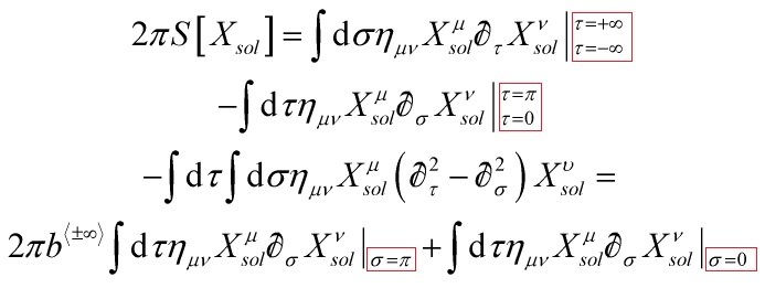
and the last two terms vanish for the Neumann boundary conditions. However, one needs to derive an nontrivial effective action for the string in the limit where its length tends to zero and hence can be modeled as a ‘particle’. To perform such a zoom-out properly, one’s instinct is to integrate the degrees of freedom along the string length: alas, this is not possible if we specify the Neumann conditions on both endpoints of the string. One ought then to define one of the string-endpoints via a Dirichlet boundary condition, plug the corresponding solution  back into
and integrate over the length parameter σ. So we get an effective action ![S\left[ {\bar X} \right]](https://www.georgeshiber.com/wp-content/ql-cache/quicklatex.com-04d536cfee5ebaf376b097052931fe77_l3.png "Rendered by QuickLaTeX.com") that hence encodes the degrees of freedom we are looking for. They correspond to a ‘particle’, but not in the usual sense of a pointwise object with local dynamics. Let’s delve deeper.
that hence encodes the degrees of freedom we are looking for. They correspond to a ‘particle’, but not in the usual sense of a pointwise object with local dynamics. Let’s delve deeper.
One Fourier transforms  in the worldsheet coordinate
  :
:
![\[{X^\mu }\left( {\tau ,\sigma } \right) = \int_{ - \infty }^{ + \infty } {\frac{{{\rm{d}}k}}{{2\pi }}} {e^{ik\tau }}g\left( {k,\sigma } \right){x^\mu }\left( k \right)\]](https://www.georgeshiber.com/wp-content/ql-cache/quicklatex.com-4da5cd48eeb15040b263124ab12b4221_l3.png "Rendered by QuickLaTeX.com")
with
![\[\left\{ {\begin{array}{*{20}{c}}{{x^\mu }\left( k \right): = \int_{ - \infty }^{ + \infty } {{\rm{d}}\tau '{e^{ - ik\tau '}}{x^\mu }\left( {\tau '} \right)} }\\{{x^\mu }\left( \tau \right): = {X^\mu }\left( {\tau ,0} \right)}\end{array}} \right.\]](https://www.georgeshiber.com/wp-content/ql-cache/quicklatex.com-28de41f9d0910740ea1a012a21643e25_l3.png "Rendered by QuickLaTeX.com")
According to
![\[{x^\mu }\left( \tau \right): = {X^\mu }\left( {\tau ,0} \right)\]](https://www.georgeshiber.com/wp-content/ql-cache/quicklatex.com-ba80b769442e8c3e6830beb1d44beef3_l3.png "Rendered by QuickLaTeX.com")
and in light of the fact that
![\[{\not \partial _\sigma }{X^\mu }\left( {\tau ,\pi } \right) = 0\]](https://www.georgeshiber.com/wp-content/ql-cache/quicklatex.com-96dc48b100b01f733f8eade5a2a08f16_l3.png "Rendered by QuickLaTeX.com")
we have:
![\[\left\{ {\begin{array}{*{20}{c}}{g\left( {k,0} \right) = 1}\\{{{\not \partial }_\sigma }g\left( {k,\sigma } \right)\left| {_{\sigma = \pi } = 0} \right.}\end{array}} \right.\]](https://www.georgeshiber.com/wp-content/ql-cache/quicklatex.com-1527bff0c9847f1595ba52ebdc8a4a59_l3.png "Rendered by QuickLaTeX.com")
Now, apply equation
to
which yields the harmonic oscillator:
![\[\left( {\not \partial _\sigma ^2 + {k^2}} \right)g\left( {k,\sigma } \right) = 0\]](https://www.georgeshiber.com/wp-content/ql-cache/quicklatex.com-4ce9a9e73bf4f3bc0a0c65fdd4f75dd3_l3.png "Rendered by QuickLaTeX.com")
with solution
![\[g\left( {k,\sigma } \right) = b_k^{\left\langle { \pm \infty } \right\rangle }\sin \left( {k\sigma } \right) + {c_k}\cos \left( {k\sigma } \right)\]](https://www.georgeshiber.com/wp-content/ql-cache/quicklatex.com-f05ae94d05946b5b92e91c7a7b137244_l3.png "Rendered by QuickLaTeX.com")
Hence, the solution of
is thus
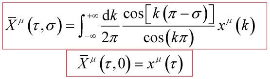
(A)
So we get the classic free-string solution:
![\[X_{{\rm{Neu}}}^\mu = {p^\mu }\tau + \sum\limits_{n \in \mathbb{Z}} {{e^{in\tau }}} \cos \left( {n\sigma } \right){x^\mu }\left( n \right)\]](https://www.georgeshiber.com/wp-content/ql-cache/quicklatex.com-ee22c459e96cd10973fcb620adf93c63_l3.png "Rendered by QuickLaTeX.com")
which when k = n, coincides with (A). However, momenta k are continuous since the function  is not a Cauchy-information-datum. So equation (A) represents a string where the σ = π endpoint are free and not bound to any brane. To extract a physical interpretation from (A), one must plug it into
and integrate over σ, and hence, that allows us to get an effective action for the endpoint coordinate  which is physically interpretable as a worldline whose dynamics is characterized by a nonlocal form-factor:
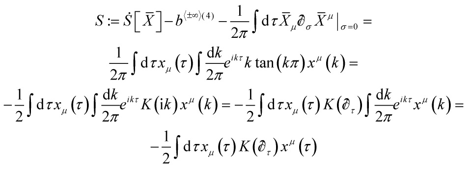
(B)
with
![\[\left\{ {\begin{array}{*{20}{c}}{K\left( {{\rm{i}}k} \right) = - \frac{1}{\pi }\tan \left( {\pi k} \right)k}\\{K\left( {{{\not \partial }_\tau }} \right) = \frac{1}{\pi }\tan \left( {\pi {{\not \partial }_\tau }} \right){{\not \partial }_\tau }}\end{array}} \right.\]](https://www.georgeshiber.com/wp-content/ql-cache/quicklatex.com-aba45b892efa55df85b5d93afd9797c4_l3.png "Rendered by QuickLaTeX.com")
and so we get
![\[S \simeq {S_{\rm{p}}} = - \frac{1}{2}\int {{\rm{d}}\tau } {x_\mu }\left( \tau \right)\not \partial _\tau ^2{x^\mu }\left( \tau \right)\]](https://www.georgeshiber.com/wp-content/ql-cache/quicklatex.com-8ec4442c94f8b8bef596e1fc22c36d85_l3.png "Rendered by QuickLaTeX.com")
which can always be picked by a worldline reparametrization and thus interpreted as a relativistic particle in the gauge of unit D-velocity, which implies that
![\[K\left( {{{\not \partial }_\tau }} \right)\delta {x^\mu } = 0 \Rightarrow K\left( {{{\not \partial }_\tau } + {\rm{i}}k} \right){\not \partial _\tau }{x^\mu } = 0\]](https://www.georgeshiber.com/wp-content/ql-cache/quicklatex.com-78d7391565e81f9ba6b2213b13b20285_l3.png "Rendered by QuickLaTeX.com")
And so, by Noether’s theorem, the conserved charges associated with this symmetry are
![\[{L_n} = \frac{1}{2}\int_{ - \pi }^{ + \pi } {{\rm{d}}\tau {e^{{\rm{i}}n\tau }}} {p_\mu }\left( \tau \right){p^\mu }\left( \tau \right)\]](https://www.georgeshiber.com/wp-content/ql-cache/quicklatex.com-51907a94869b28c3b91f3b6849ff5e42_l3.png "Rendered by QuickLaTeX.com")
with:
![\[{p^\mu }: = \delta S/\delta \left( {{{\not \partial }_\tau }{x^\mu }} \right)\]](https://www.georgeshiber.com/wp-content/ql-cache/quicklatex.com-76d1e90858a4f1e08ee37c162f83c78e_l3.png "Rendered by QuickLaTeX.com")
the conjugate momentum, and  obey a Virasoro algebra with vanishing central charge.
The infinite countable number of modes of the string are all contained in the operator 
So, define the nonlocal operator  such that
![\[K = {\not \partial _\tau }\left( {{f_0}{{\not \partial }_\tau } \cdot } \right)\]](https://www.georgeshiber.com/wp-content/ql-cache/quicklatex.com-e4163c122d711c55461ac4ba3365e636_l3.png "Rendered by QuickLaTeX.com")
and so, by integrating-by-parts, the action (B) above reduces to:
![\[S = \frac{1}{2}\int {{\rm{d}}\tau } \left( {{{\not \partial }_\tau }{x_\mu }} \right){f_0}\left( {{{\not \partial }_\tau }} \right){\not \partial _\tau }{x^\mu }\]](https://www.georgeshiber.com/wp-content/ql-cache/quicklatex.com-15e6534ca54c5b4e46c1689dadae434d_l3.png "Rendered by QuickLaTeX.com")
and note that the inverse operator  admits the series representation
![\[\frac{1}{{{f_0}\left( {{{\not \partial }_\tau }} \right)}} = 1 + 2\sum\limits_{n = 1}^{ + \infty } {\frac{{\not \partial _\tau ^2}}{{\not \partial _\tau ^2 + {n^2}}}} \]](https://www.georgeshiber.com/wp-content/ql-cache/quicklatex.com-010ef1e6c7e4911fcbfb369b83805c12_l3.png "Rendered by QuickLaTeX.com")
Thus recasting  as an infinite superposition of modes
as an infinite superposition of modes ![\[{x^\mu }\left( \tau \right) = x_0^\mu \left( \tau \right) + 2\sum\limits_{n = 1}^{ + \infty } {x_n^\mu } \left( \tau \right)\]](https://www.georgeshiber.com/wp-content/ql-cache/quicklatex.com-5d3565db20f364b2033849774693bcdf_l3.png "Rendered by QuickLaTeX.com")
with:
![\[\left\{ {\begin{array}{*{20}{c}}{x_0^\mu : = {f_0}\left( {{{\not \partial }_\tau }} \right){x^\mu }}\\{x_n^\mu : = \frac{{\not \partial _\tau ^2}}{{\not \partial _\tau ^2 + {n^2}}}{f_0}\left( {{{\not \partial }_\tau }} \right){x^\mu }}\end{array}} \right.\]](https://www.georgeshiber.com/wp-content/ql-cache/quicklatex.com-a450b8f3d2796b588ac6c5dfb173f0e2_l3.png "Rendered by QuickLaTeX.com")
Hence, up to a total derivative,
becomes:
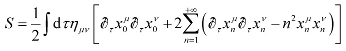
And upon quantization, (B) is unitary with positive semidefinite Hamiltonian  , and the generators
  obey the Virasoro algebra
, and the generators obey the Virasoro algebra ![\[\begin{array}{c}\left[ {{{\hat L}_m},{{\hat L}_n}} \right] = \left( {m - n} \right){{\hat L}_{m + n}} - \\\left( {c/12} \right)m\left( {{m^2} - 1} \right){\delta _{m + n,0}}\end{array}\]](https://www.georgeshiber.com/wp-content/ql-cache/quicklatex.com-573814836d8b1498022d93bd76990257_l3.png "Rendered by QuickLaTeX.com")
with
![\[{\hat L_n} = \left( {1/2} \right){\eta _{\mu \nu }}\sum\nolimits_{m \in \mathbb{Z}} {y_{n - m}^\mu } y_m^\nu \]](https://www.georgeshiber.com/wp-content/ql-cache/quicklatex.com-044455d0f722a2c9df30ed4704bf28e4_l3.png "Rendered by QuickLaTeX.com")
Hence, the infinite number of degrees of freedom encoded in the nonlocal action (B) are nothing but the open bosonic string spectrum. The nonlocal model realizes the same Fock space of physical states of the full theory, and the Polyakov action yields a nonlocal theory for a zoomed-out string which ‘looks’ like a particle at the zoom-limit = 0


2 Responses
String-Theory and Calabi-Yau Fourfolding of M-Theory
Monday, July 18, 2016[…] GUT, such 4-D compactifications are essential in order to have a correspondence with 4-D spacetime. Recall I derived, via Clifford algebraic symmetry, the total […]
The String-String Duality, K3 Geometry, and Dimensional Reduction
Wednesday, November 23, 2016[…] Recall I derived, via Clifford algebraic symmetry, the total action: […]