The cosmological primordial perturbations of the universe, implicitly defined by the Wheeler–DeWitt equation:
![\[\begin{array}{l}\tilde H\Psi = \left( {\frac{{2\pi G{\hbar ^2}}}{3}} \right.\frac{{{\partial ^2}}}{{\partial {\alpha ^2}}} - \frac{{{\hbar ^2}}}{2}\frac{{{\partial ^2}}}{{\partial {\phi ^2}}}\\ + \,{e^{6\alpha }}\left( {V\left( \phi \right) + \frac{\Lambda }{{8\pi G}}} \right) - 3{e^{4\alpha }}\left. {\frac{k}{{8\pi G}}} \right)\Psi \left( {\alpha ,\phi } \right) = 0\end{array}\]](https://www.georgeshiber.com/wp-content/ql-cache/quicklatex.com-8e996abafc46629c4ce4962e1ac63a4c_l3.png "Rendered by QuickLaTeX.com")
a partial differential equation determining a wave-function not defined in space or time or spacetime, with:
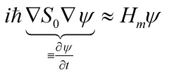
![\[\Psi { \approx _{Heisb}}\exp \left( {i{S_0}\left[ {{h_{ab}}} \right]/\hbar } \right)\psi \left[ {{h_{ab}},\left\{ {{x_n}} \right\}} \right]\]](https://www.georgeshiber.com/wp-content/ql-cache/quicklatex.com-caaffd0631ab0f16e8e9886a6aebe56f_l3.png "Rendered by QuickLaTeX.com")
and  satisfies an approximate Schrödinger equation:
are clearly quantum in origin. One of the central foundational philosophically pressing problems in physics is to describe a ‘collapse’ dynamics that explains the classical features consistent with astrophysical data. Given the ‘no-time’-property of the Wheeler–DeWitt equation: namely, that it lacks an external time parameter and it lacks a first derivative with an imaginary Schrödinger time-factor, as well as its linearity and symmetrization, we face a deep conflict with the Lindblad equation:
![\[\begin{array}{l}\frac{{d{{\hat \rho }_S}}}{{dt}} = - \frac{i}{\hbar }\left[ {{{\hat H}_S},\hat \rho } \right] + \\\gamma \sum\limits_j {\left[ {{{\hat L}_j}{{\hat \rho }_S}\hat L_j^\dagger - \frac{1}{2}\left\{ {\hat L_j^\dagger {{\hat L}_j},{{\hat \rho }_S}} \right\}} \right]} \end{array}\]](https://www.georgeshiber.com/wp-content/ql-cache/quicklatex.com-6bc4664bb0862d7eb83dc7d2db66936a_l3.png "Rendered by QuickLaTeX.com")
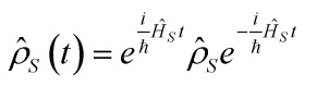
given that its central properties are time-asymmetry and entanglement-entropic-irreversibility, and whose Lindbladian:
![\[\gamma \left[ {\hat S{{\hat \rho }_S}{{\hat S}^\dagger } - \frac{1}{2}\left\{ {{{\hat S}^\dagger }\hat S,{{\hat \rho }_S}} \right\}} \right]\]](https://www.georgeshiber.com/wp-content/ql-cache/quicklatex.com-268b769d7fb353b409ab47251168c520_l3.png "Rendered by QuickLaTeX.com")
describes the non-unitary evolution of the density operator, with:
![\[\gamma \equiv 2\pi \int_0^\infty {d\omega J\left( \omega \right)\delta \left( \omega \right)} \]](https://www.georgeshiber.com/wp-content/ql-cache/quicklatex.com-b157f63d8726859ebc8594bf2b232f34_l3.png "Rendered by QuickLaTeX.com")
Besides the problem of the undefinability of the Lindbladian system-bath interaction:
![\[\left\{ {\begin{array}{*{20}{c}}{{{\hat H}_{SB}} = \hbar \left( {\hat S{{\hat B}^\dagger } + {{\hat S}^\dagger }\hat B} \right)\quad }\\{{{\hat H}_B} = \hbar \sum\limits_k {{\omega _k}\hat a_k^\dagger } {{\hat a}_k}}\end{array}} \right.\]](https://www.georgeshiber.com/wp-content/ql-cache/quicklatex.com-e592e405451fbe9a05e7f86ed5570945_l3.png "Rendered by QuickLaTeX.com")
and
![\[\left\{ {\begin{array}{*{20}{c}}{\left[ {\hat S,{{\hat H}_S}} \right] = 0}\\{\hat S\left( t \right) = \hat S\quad ;\quad \hat B = \sum\limits_k {g_k^ * } {{\hat a}_k}}\\{\hat B\left( t \right) = {e^{\frac{i}{\hbar }{{\hat H}_B}t}}\hat B{e^{ - \,\frac{i}{\hbar }{{\hat H}_B}t}}}\end{array}} \right.\]](https://www.georgeshiber.com/wp-content/ql-cache/quicklatex.com-7651b23d2cf65471dfe1f5eaa8ebdf8e_l3.png "Rendered by QuickLaTeX.com")
in the quantum gravitational cosmology context: see Derivation of the Lindblad Equation for technical details, we already face the tripartite conflict of time, which borders on the paradoxical, and is one of the main reasons, outside of M-theory, why quantum gravity theories are unviable. Now, clearly that restricts and limits our theories of wave-functional collapse. My aim here is to show how spontaneous collapse dynamics provides such an explanation, and moreover, with essential use of the k−inflationary action:
![\[\begin{array}{*{20}{l}}{S = - \frac{1}{{16\pi G}}\int {{d^4}} x\sqrt { - g} R + }\\{\int {{d^4}} x\sqrt { - g} p\left( {X,\varphi } \right)}\end{array}\]](https://www.georgeshiber.com/wp-content/ql-cache/quicklatex.com-569c270a7e820cce3562ff90d38bb098_l3.png "Rendered by QuickLaTeX.com")
of consequence since the inflaton field is an essential feature of the primordial quantum-to-classical collapse-transition. With
![\[X \equiv \frac{1}{2}{g^{\mu \nu }}{\partial _\mu }\varphi \,{\not \partial _\nu }\varphi \]](https://www.georgeshiber.com/wp-content/ql-cache/quicklatex.com-9d4b93449c59c0ce66f58ac8cad88afa_l3.png "Rendered by QuickLaTeX.com")
the canonical inflaton kinetic term, and the matter Lagrangian  can be varied with respect to the metric to yield the energy-momentum tensor of the inflaton field:
![\[{T_{\mu \nu }} = \left( {\varepsilon + p} \right){w_\mu }{w_\nu } - p{g_{\mu \nu }}\]](https://www.georgeshiber.com/wp-content/ql-cache/quicklatex.com-a27a2d1596da0b72a48842e3e0033c4d_l3.png "Rendered by QuickLaTeX.com")
with energy density being  ,
,  the Lagrangian of the scalar field and
  .
.
In a flat Friedmann-Robertson-Walker metric as the background geometry, the above Lagrangian gives us the standard Friedmann equations:
![\[\left\{ {\begin{array}{*{20}{c}}{{H^2} = \frac{1}{{3M_{{\rm{PI}}}^2}}\varepsilon }\\{\dot H = - \frac{1}{{3M_{{\rm{PI}}}^2}}\left( {\varepsilon + p} \right)}\end{array}} \right.\]](https://www.georgeshiber.com/wp-content/ql-cache/quicklatex.com-440e15f34b464794d1b3d1e7158ed390_l3.png "Rendered by QuickLaTeX.com")
and continuity equation as:
![\[\dot \varepsilon = - 3H\left( {\varepsilon + p} \right)\]](https://www.georgeshiber.com/wp-content/ql-cache/quicklatex.com-9833b3353c01ff98c6769ebd01c282bb_l3.png "Rendered by QuickLaTeX.com")
 the Hubble parameter,
  is derivative with respect to cosmic time
  and
and  the reduced Planck mass, from which we can derive the following:
![\[\begin{array}{l}\dot p = - 3c_s^2H\left( {\varepsilon + p} \right) + \\\dot \varphi \left( {{p_{,\varphi }} - c_s^2{\varepsilon _{,\varphi }}} \right)\end{array}\]](https://www.georgeshiber.com/wp-content/ql-cache/quicklatex.com-b5b21b7b1501ce586673dd7c4346d28b_l3.png "Rendered by QuickLaTeX.com")
and the parameter  is given by:
![\[c_s^2 \equiv \frac{{p,X}}{{{\varepsilon _{,X}}}} = \frac{{\varepsilon + p}}{{2X{\varepsilon _{,X}}}}\]](https://www.georgeshiber.com/wp-content/ql-cache/quicklatex.com-f2674ea6448e70058abc406f113a0d3a_l3.png "Rendered by QuickLaTeX.com")
and is the upper limit on the inflationary perturbations cosmic-speed.
The key reason why k−inflationary cosmology is of import is the implementation of the inflation-phase even when the potential of the inflaton-field either tends to zero or grows very fast, barring slow-rolls. The k−inflation Lagrangian  vanishes as
  and in the
  -region, we can expand it as:
![\[\begin{array}{l}p\left( {\varphi ,X} \right) = K\left( \varphi \right)X + L\left( \varphi \right){X^2}\\ + ...\end{array}\]](https://www.georgeshiber.com/wp-content/ql-cache/quicklatex.com-4addf3e3bc310787904700193e3dda7b_l3.png "Rendered by QuickLaTeX.com")
and given that the Lagrangian is a function of the pure kinetic term  , it follows that the evolution equation tends towards an attractor
  , hence leading to a pure exponential expansion of the universe as required to drive inflation dynamics. Let us deal with the graceful-exit problem. In the limit, we have:
![\[p\left( {\varphi ,X} \right) = K\left( \varphi \right)X + L\left( \varphi \right){X^2}\]](https://www.georgeshiber.com/wp-content/ql-cache/quicklatex.com-0020a0ceeec465ce97e77a1096c02c6d_l3.png "Rendered by QuickLaTeX.com")
![\[\varepsilon \left( {\varphi ,X} \right) = K\left( \varphi \right)X + 3L\left( \varphi \right){X^2}\]](https://www.georgeshiber.com/wp-content/ql-cache/quicklatex.com-b0f673a66ef86562e13ec88f0db2a259_l3.png "Rendered by QuickLaTeX.com")
If the coefficients  ,
,  are positive, our Lagrangian would fail to lead to an inflationary solution. In the case of
  , solutions tend toward an inflationary fixed-point
  , constructible as such: at fixed point
  , we have
  . One can take
  without any loss of generality, which yields the 0-th order slow-roll quantities:
![\[\left\{ {\begin{array}{*{20}{c}}{{X_{sr}} = \frac{1}{2}\tilde K\left( {{\varphi _{sr}}} \right)}\\{{\varepsilon _{sr}} = \frac{1}{4}{{\tilde K}^2}\left( {{\varphi _{sr}}} \right)}\\{{H_{sr}} = {{\left( {2\sqrt 3 {M_{{\rm{PI}}}}} \right)}^{ - 1}}\tilde K\left( {{\varphi _{sr}}} \right)}\end{array}} \right.\]](https://www.georgeshiber.com/wp-content/ql-cache/quicklatex.com-838641f17ea617ff325f374d62fb5263_l3.png "Rendered by QuickLaTeX.com")
giving us:
![\[\left\{ {\begin{array}{*{20}{c}}{\delta X/{X_{sr}} \ll 1}\\{\partial {{\left( {\tilde K} \right)}^{ - 1/2}}/\partial \varphi \ll 3/2}\end{array}} \right.\]](https://www.georgeshiber.com/wp-content/ql-cache/quicklatex.com-e85c9e0907707a21a9f2c2f9aca0e43b_l3.png "Rendered by QuickLaTeX.com")
The Hubble k−inflation-slow-roll parameters are:
![\[\left\{ {\begin{array}{*{20}{c}}{{\varepsilon _0} = - \frac{{\dot H}}{{{H^2}}}}\\{{\varepsilon _{n + 1}} = \frac{{\dot \varepsilon }}{{H{\varepsilon _n}}}}\end{array}} \right.\]](https://www.georgeshiber.com/wp-content/ql-cache/quicklatex.com-dfd41f46b6bd5fb39db71c0dd0f0934b_l3.png "Rendered by QuickLaTeX.com")
and constrained by:
![\[\left\{ {\begin{array}{*{20}{c}}{{\varepsilon _0} = \left( {3/2} \right)\left( {1 + p/\varepsilon } \right)}\\{{\varepsilon _1} = {H^{ - 1}}\left( {{\rm{In}}\left( {1 + p/\varepsilon } \right)} \right)}\\{{s_0} = {H^{ - 1}}\left( {{\rm{In}}\left( {{c_s}} \right)} \right)}\end{array}} \right.\]](https://www.georgeshiber.com/wp-content/ql-cache/quicklatex.com-d35c583b42e0bd9dec5441827b5a0c74_l3.png "Rendered by QuickLaTeX.com")
Such a model needs only two scalar perturbation terms: the inflaton fluctuation  and the metric perturbation
  . Note that such a choice of gauge has the property that the scalar perturbations are the same as the gauge invariant quantities: gauge invariant inflaton perturbations and the Bardeen potential respectively. We now define a gauge-invariant scalar
  from and as such:
![\[\zeta = \Phi + H\frac{{\delta \varphi }}{{\dot \varphi }}\]](https://www.georgeshiber.com/wp-content/ql-cache/quicklatex.com-51ea4ae80a23f81f18f426d6157d06d3_l3.png "Rendered by QuickLaTeX.com")
which is equivalent to the comoving curvature perturbation  in this gauge, yielding the desired action:
![\[S = \frac{1}{2}\int {{z^2}} \left[ {{{\zeta '}^2} + c_s^2\zeta \,{\partial _i}{\partial ^i}\zeta } \right]d\tau {d^3}x\]](https://www.georgeshiber.com/wp-content/ql-cache/quicklatex.com-24ea215b2d7b5052dff994819d3659b3_l3.png "Rendered by QuickLaTeX.com")
with  the conformal time and
  is defined by:
![\[z = \frac{{a\sqrt {\varepsilon + p} }}{{{c_s}H}} = \frac{{a{M_{{\rm{PI}}}}}}{{{c_s}}}\sqrt {2{\varepsilon _0}} \]](https://www.georgeshiber.com/wp-content/ql-cache/quicklatex.com-f347b1c32492074894d4bc5d32c6fc96_l3.png "Rendered by QuickLaTeX.com")
We now define a canonical quantization variable  and the corresponding action is hence:
![\[S = \frac{1}{2}\int {\left[ {{{\upsilon '}^2} + c_s^2\upsilon {\partial _i}{\partial ^i}\upsilon + \frac{{z''}}{z}{\upsilon ^2}} \right]} {\mkern 1mu} d\tau {d^3}x\]](https://www.georgeshiber.com/wp-content/ql-cache/quicklatex.com-57857f8b6b84ce8febc5718734cf53fe_l3.png "Rendered by QuickLaTeX.com")
from which we can derive the equation of motion for  in momentum space:
![\[{\upsilon ''_k} + \left( {c_s^2{k^2} - \frac{{z''}}{z}} \right){\upsilon _k} = 0\]](https://www.georgeshiber.com/wp-content/ql-cache/quicklatex.com-1f5521d149b1e6db712eb18a0aecab29_l3.png "Rendered by QuickLaTeX.com")
with the mode function:
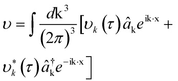
with
![\[\left[ {{{\hat a}_{\rm{k}}},\hat a_{{\rm{k'}}}^\dagger } \right] = {\left( {2\pi } \right)^3}{\delta ^3}\left( {{\rm{k}} - {\rm{k'}}} \right)\]](https://www.georgeshiber.com/wp-content/ql-cache/quicklatex.com-0431e6da5a2120c81c5043cea3c4ca4c_l3.png "Rendered by QuickLaTeX.com")
and during slow-roll
![\[z''/z \sim a''/a \sim 2{\left( {aH} \right)^2}\]](https://www.georgeshiber.com/wp-content/ql-cache/quicklatex.com-94d0d0359458670690fe7d7bf49194f6_l3.png "Rendered by QuickLaTeX.com")
a mode  crosses the sound-horizon
  when
when  . Hence, in the subhorizon limit
  we can drop the potential term
  , giving us the solution to the above equation for positive frequency mode:
![\[{\upsilon _k} \sim \frac{{{e^{ - i{c_s}k\tau }}}}{{\sqrt {2{c_s}k} }}\]](https://www.georgeshiber.com/wp-content/ql-cache/quicklatex.com-ff46a163fcc1ed5b4929a0f897fc7163_l3.png "Rendered by QuickLaTeX.com")
Now, if a mode is too much beyond the sound-horizon, the potential term dominates and the solution would be:
![\[{\upsilon _k} \sim {C_k}{z_i}\]](https://www.georgeshiber.com/wp-content/ql-cache/quicklatex.com-dbb1c9855822621133b141a2ae5f2990_l3.png "Rendered by QuickLaTeX.com")
yielding the sound-horizon coefficient:
![\[{\left| {{C_k}} \right|^2} = {\left( {2{z^{ * 2}}{c_s}k} \right)^{ - 1}}\]](https://www.georgeshiber.com/wp-content/ql-cache/quicklatex.com-3a31292247fb0351c9d82ddaec770002_l3.png "Rendered by QuickLaTeX.com")
with  the crossing-value at sound-horizon. Hence, the comoving power spectrum curvature perturbation is determined by:
![\[\begin{array}{c}P_R^ * = \frac{{{k^3}}}{{2\pi }}{\left| {R_k^ * } \right|^2} = \frac{{{k^3}}}{{2{\pi ^2}}}{\left| {\zeta _k^ * } \right|^2} = \\\frac{{{k^3}}}{{2{\pi ^2}{z^{ * 2}}}}{\left| {\upsilon _k^ * } \right|^2}\end{array}\]](https://www.georgeshiber.com/wp-content/ql-cache/quicklatex.com-14facf507260a48b4f2aca2245998f65_l3.png "Rendered by QuickLaTeX.com")
more informatively expanded as:
![\[\begin{array}{c}P_R^ * = \frac{1}{{8{\pi ^2}}}\frac{{{H^2}}}{{{\varepsilon _0}{c_s}M_{{\rm{PI}}}^2}}{\left( {\frac{k}{{{k_{\rm{P}}}}}} \right)^{{n_s} - 1}} \equiv \\{A_s}{\left( {\frac{k}{{{k_{\rm{P}}}}}} \right)^{{n_s} - 1}}\end{array}\]](https://www.georgeshiber.com/wp-content/ql-cache/quicklatex.com-70480479c67d3e9f99f5a5effb1281c6_l3.png "Rendered by QuickLaTeX.com")
where  is the Planck pivot, and is given by
  . The scalar spectral index
  measures the scale dependence of the scalar spectrum, which depends on the slow-roll parameters as:
![\[{n_s} - 1 = \frac{{d{\rm{In}}{P_R}}}{{d{\rm{In}}k}} = - 2{\varepsilon _0} - {\varepsilon _1} - {s_0}\]](https://www.georgeshiber.com/wp-content/ql-cache/quicklatex.com-012a561288c9cbfadd09571e47fee269_l3.png "Rendered by QuickLaTeX.com")
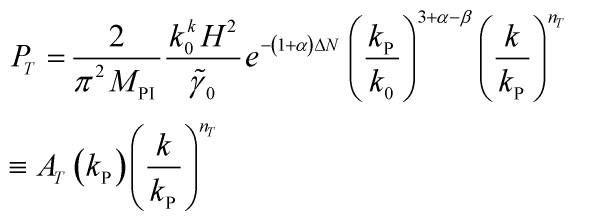
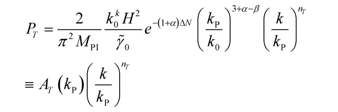
The tensor metric perturbations generated during k−inflation dynamically evolve, and escape the horizon when  . So the tensor power spectrum is:
![\[\begin{array}{*{20}{c}}{{P_T} = \frac{2}{{{\pi ^2}}}\frac{{{H^2}}}{{M_{{\rm{PI}}}^2}}{{\left( {\frac{k}{{{k_{\rm{P}}}}}} \right)}^{{n_T}}} \equiv }\\{{A_T}{{\left( {\frac{k}{{{k_{\rm{P}}}}}} \right)}^{{n_T}}}}\end{array}\]](https://www.georgeshiber.com/wp-content/ql-cache/quicklatex.com-7bbf4fa5235465275e094553550de54e_l3.png "Rendered by QuickLaTeX.com")
with spectral index:
![\[{n_T} = - 2{\varepsilon _0}\]](https://www.georgeshiber.com/wp-content/ql-cache/quicklatex.com-e01eabec2b8d34303dbe36087e471145_l3.png "Rendered by QuickLaTeX.com")
Now, the central quantity to be measured is the tensor-to-scalar ratio
![\[\tau \equiv {A_T}/{A_s}\]](https://www.georgeshiber.com/wp-content/ql-cache/quicklatex.com-fefd3dcbb2643f9241ba4405c5af67ca_l3.png "Rendered by QuickLaTeX.com")
which the k−inflationary scenario predicts as:
![\[\tau = - 8{c_s}{n_T}\]](https://www.georgeshiber.com/wp-content/ql-cache/quicklatex.com-20f7763f7ceea5cf0eece6c26644723f_l3.png "Rendered by QuickLaTeX.com")
Collapse models in quantum mechanics must modify the Schrödinger equation phenomenologically by adding non-linear stochastic terms in order to break wavefunctional-superposition and to explain the stochastic outcomes of fully deterministic evolutionary equation
The non-linear evolution is norm-preserving and the stochastic evolution obeys the Born probability rule. An initial and fundamental problem is that there are a plethora of collapse-models, an embarrassment of riches problem, that also gives rise to the philosophical problem of underdetermination. As mentioned above, the standard models, certainly and especially the Copenhagen model, are inadequate. In the quantum cosmological picture, the Continuous Spontaneous Localization (CSL) model of Ghirardi-Pearle-Rimini is the one that is adequate and can account for all the aspects of a quantum-cosmological collapse model, and mainly due to the amplification property that yields a collapse-parameter  that scales as the total mass of the system so that the localization is stronger for larger system. The modified CSL-Schrödinger equation is given as:
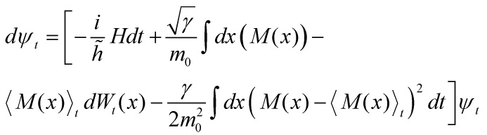
and the first term on the right hand side is the linear term of the Schrödinger equation and the next two terms are the stochastic and non-linear ones respectively, and where  is the Wiener process that encodes the stochasticity of the evolution,
  is the smeared mass density operator.
- The question now is how can the CSL-collapse mechanism be implemented in a canonical inflationary scenario.
In single-field canonical slow-rolls, the two scalar perturbations and yield the Mukhanov-Sasaki variable  , which is a gauge-invariant quantity, and is:
![\[{\zeta _{{\rm{MS}}}} = \delta \varphi + \frac{{\dot \varphi }}{H}\Phi \]](https://www.georgeshiber.com/wp-content/ql-cache/quicklatex.com-0b3691a2695108135ac59d7419dc9ba3_l3.png "Rendered by QuickLaTeX.com")
Now, define
![\[{\tilde \zeta _{{\rm{MS}}}} \equiv a{\zeta _{{\rm{MS}}}}\]](https://www.georgeshiber.com/wp-content/ql-cache/quicklatex.com-9b42995170d9684ffc94484ebbe9fb23_l3.png "Rendered by QuickLaTeX.com")
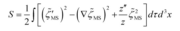
and we get the action:
with  . Now, the wavefunctional of the variable
  in momentum space is:
![\[\begin{array}{l}\Psi \left[ {{{\tilde \zeta }_{{\rm{MS}}}}} \right] = \sum\limits_{\rm{k}} {\Psi _{\rm{k}}^{\rm{R}}} \left[ {\tilde \zeta _{{\rm{M}}{{\rm{S}}_{\rm{k}}}}^{\rm{R}}\left( \tau \right)} \right] \cdot \\\Psi _{\rm{k}}^{\rm{I}}\left[ {\tilde \zeta _{{\rm{M}}{{\rm{S}}_{\rm{k}}}}^{\rm{I}}\left( \tau \right)} \right]\end{array}\]](https://www.georgeshiber.com/wp-content/ql-cache/quicklatex.com-336e586910c8c2eeaa242fbc59d7224d_l3.png "Rendered by QuickLaTeX.com")
and satisfies the CSL-modified Schrödinger equation functional:
and has the same form as the CSL-modified Schrödinger equation given in equation:
The Hamiltonian then takes the form of a simple harmonic oscillator:
with a time-dependent frequency
![\[{\omega ^2}\left( {\tau ,k} \right) = {k^2} - a''/a\]](https://www.georgeshiber.com/wp-content/ql-cache/quicklatex.com-a93770c6e1f11bb665605a0876f01238_l3.png "Rendered by QuickLaTeX.com")
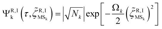
due to background expansion. The key is that this functional Schrödinger equation has a Gaussian functional as a solution to:
with:
![\[\left| {{N_k}} \right| = {\left( {{\mathop{\rm Re}\nolimits} {\Omega _k}/\pi } \right)^{1/2}}\]](https://www.georgeshiber.com/wp-content/ql-cache/quicklatex.com-a53c947b127c3f8a0da3365c609c03b1_l3.png "Rendered by QuickLaTeX.com")
and  satisfies the following differential equation:
![\[{\Omega '_k} = - i\Omega _k^2 + i{\tilde \omega ^2}\left( {\tau ,k} \right)\]](https://www.georgeshiber.com/wp-content/ql-cache/quicklatex.com-3ff0e038ae21d42996b054bbd9631675_l3.png "Rendered by QuickLaTeX.com")
where the following holds:
![\[{\tilde \omega ^2} = {\omega ^2} - 2i\gamma \]](https://www.georgeshiber.com/wp-content/ql-cache/quicklatex.com-356f7a9ee9b73ff82095a1154b3d6981_l3.png "Rendered by QuickLaTeX.com")
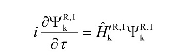
Hence, the wavefunction of the Mukhanov-Sasaki variable satisfy the Schrödinger equation:
with the following Gaussian solution:
and for the correlation function of the Mukhanov-Sasaki variable in the Schrödinger picture, we have:
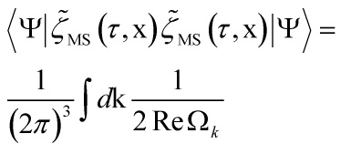
with power spectrum:
![\[{P_{{{\tilde \zeta }_{{\rm{MS}}}}}} = \frac{{{k^3}}}{{4{\pi ^2}}}\frac{1}{{{\mathop{\rm Re}\nolimits} {\Omega _k}}}\]](https://www.georgeshiber.com/wp-content/ql-cache/quicklatex.com-260ce30698ce6753484eaf0d5a3ffa9b_l3.png "Rendered by QuickLaTeX.com")
and the comoving curvature perturbations power spectrum is:
![\[{P_R} = \frac{{{k^3}}}{{8{\pi ^2}{\varepsilon _0}M_{{\rm{PI}}}^2}}\frac{1}{{{a^2}{\mathop{\rm Re}\nolimits} {\Omega _k}}}\]](https://www.georgeshiber.com/wp-content/ql-cache/quicklatex.com-ae6869aed320c75efb7b5b93a3f58c57_l3.png "Rendered by QuickLaTeX.com")
where we implicitly used:
![\[{\varepsilon _V} \equiv \left( {1/2M_{{\rm{PI}}}^{\rm{2}}} \right){\left( {V'/V} \right)^2} \sim {\varepsilon _0}\]](https://www.georgeshiber.com/wp-content/ql-cache/quicklatex.com-77aba3fa90676f7a15262c021d42ea42_l3.png "Rendered by QuickLaTeX.com")
In the Heisenberg picture, in order to determine  , we decompose
  in terms of mode-functions
  as:
as:
![\[{\tilde \zeta '_{{\rm{M}}{{\rm{S}}_{\rm{k}}}}} = {f_k}\left( \tau \right){\hat a_k}\left( \tau \right) + f_k^ * \left( \tau \right)\hat a_{ - k}^\dagger \left( \tau \right)\]](https://www.georgeshiber.com/wp-content/ql-cache/quicklatex.com-74d6de552c8386c6f793f3345ef01632_l3.png "Rendered by QuickLaTeX.com")
satisfying the following two equations:
![\[\left\{ {\begin{array}{*{20}{c}}{{f_k}f_k^{ * '} - f_k^ * {{f'}_k} = i}\\{{\Omega _k} = - if_k^{ * '}/f_k^ * }\end{array}} \right.\]](https://www.georgeshiber.com/wp-content/ql-cache/quicklatex.com-e44bfc4ac8fe26a0ab54272f5c0225e1_l3.png "Rendered by QuickLaTeX.com")
and in both, the Heisenberg and Schrödinger pictures, we have:
![\[{f''_k} - {\omega ^2}{f_k} = 0\]](https://www.georgeshiber.com/wp-content/ql-cache/quicklatex.com-e52dc15dfa4e8877bb4f52a27354d8f9_l3.png "Rendered by QuickLaTeX.com")
as well as:
![\[{\mathop{\rm Re}\nolimits} {\Omega _k} = 1/2{\left| {{f_k}} \right|^2}\]](https://www.georgeshiber.com/wp-content/ql-cache/quicklatex.com-dc9e09e079c9b54f34d0b4a1573c5046_l3.png "Rendered by QuickLaTeX.com")
We need now to determine the form of the collapse parameter . It should only be determined by how the modes become classical in the presence of the collapse dynamics. The classicality of a mode is defined by its form as determined by the Wigner function, which is the correlation of the field amplitude and its conjugate momentum:
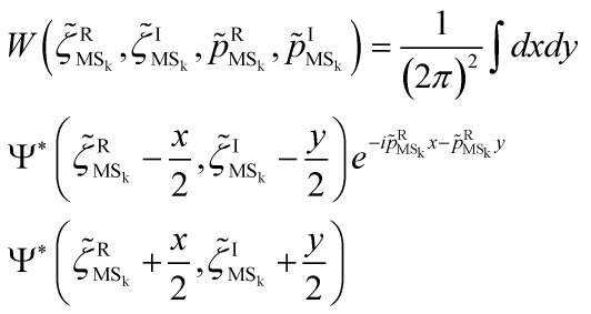
Solving, the wavefunctional is then:
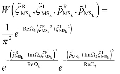
Since the Wigner function is a product of four Gaussians, two for the field amplitudes and two for its conjugate momentum, in a canonical single-field slow-roll inflationary scenario, with no collapse dynamics, we have  on superhorizon scales, squeezing the Wigner function in the momentum direction and spreading it in the field direction
hence a canonical inflationary scenario cannot explain the localization of the initial cosmological perturbations in the field variable
The solution lies in eliminating the condition  for superhorizon modes so that the Wigner function gets squeezed in the field direction so as to explain the localization, thus classicalization, of the primordial perturbations consistent with CMBR data, and for CSL-collapse dynamics, the collapse parameter must be a constant, with the condition that
  . Since the inflationary fluctuations are quantum while they are sub-horizon and become more and more squeezed, thus classical, when they start to cross the horizon to become superhorizon, it follows that the collapse of the wavefunction of the perturbations should occur during or after the primordial horizon-crossing and the collapse parameter grows with the modes. Therefore, a phenomenological form of the collapse parameter would have to be:
![\[\gamma = \frac{{{\gamma _0}\left( k \right)}}{{{{\left( { - k\tau } \right)}^\alpha }}}\]](https://www.georgeshiber.com/wp-content/ql-cache/quicklatex.com-68e3772ff73359feb01f9f91e806b63c_l3.png "Rendered by QuickLaTeX.com")
with  . Now we can solve for
and we have:
![\[{\mathop{\rm Re}\nolimits} {\Omega _k} \sim \frac{k}{2}{\left( { - k\tau } \right)^{1 - \alpha }}\left( {\frac{{2{\gamma _0}\left( k \right)}}{{{k^2}}}} \right)\]](https://www.georgeshiber.com/wp-content/ql-cache/quicklatex.com-730cae8eab2e3d460eabfa9b3fb9b865_l3.png "Rendered by QuickLaTeX.com")
We still have the problem that while incorporating the amplification mechanism does help in explaining the classicalization of the primordial perturbations in the desired parameter range, we cannot choose such a collapse parameter in such a way as to yield a scale-dependent curvature power spectrum, since that is ruled out by CMBR data. To solve this acute problem, we set:
![\[{\gamma _0}\left( k \right) = {\tilde \gamma _0}{\left( {\frac{k}{{{k_0}}}} \right)^\beta }\]](https://www.georgeshiber.com/wp-content/ql-cache/quicklatex.com-7461c5fbe96479f4bbec161c8516e795_l3.png "Rendered by QuickLaTeX.com")
with  a constant and
  the comoving wave-number of the mode which is at the present-horizon
  .
.
Hence, we get the scale dependence of the curvature power as:
![\[{P_R}\left( k \right) \propto {k^{3 + \alpha - \beta }}\]](https://www.georgeshiber.com/wp-content/ql-cache/quicklatex.com-5aeca84c7dd536f189d2313898cd81db_l3.png "Rendered by QuickLaTeX.com")
with  yielding the scale-invariant spectrum satisfying the CMBR data. Hence, the curvature power spectrum and scalar spectral index become:
where  and we have:
![\[\begin{array}{c}{n_s} - 1 = 3 + \alpha - \beta + 2\eta - 4{\varepsilon _0}\\ = \delta - 2{\varepsilon _0} - {\varepsilon _1}\end{array}\]](https://www.georgeshiber.com/wp-content/ql-cache/quicklatex.com-6cc2672eef133fb0810a748356aaf23e_l3.png "Rendered by QuickLaTeX.com")
as well as:
![\[\left\{ {\begin{array}{*{20}{c}}{\eta = {\varepsilon _0} - {{\dot \varepsilon }_0}/\left( {2{H_{{\varepsilon _0}}}} \right)}\\{{\varepsilon _1} \equiv {{\dot \varepsilon }_0}/\left( {{H_{{\varepsilon _0}}}} \right)}\\{\delta \equiv 3 + \alpha - \beta }\end{array}} \right.\]](https://www.georgeshiber.com/wp-content/ql-cache/quicklatex.com-e33b2fd8e9645236b7c8fcc9778dc84a_l3.png "Rendered by QuickLaTeX.com")
Since the primordial tensor perturbations are also essentially quantum, if they are generated during inflation, one must implement the same collapse dynamics to tensor perturbations, and with no loss of generality, we can take the same collapse parameter as given by:
to generate classicalization. Hence, the tensor power spectrum and the tensor spectral index become:
and:
![\[{n_T} = \delta - 2{\varepsilon _0}\]](https://www.georgeshiber.com/wp-content/ql-cache/quicklatex.com-55514415bd958b56333e67f461976f1c_l3.png "Rendered by QuickLaTeX.com")
and the collapse dynamics modifies both the scalar and tensor spectral indices due to the term  .
.
If  , a fair assumption, then is a non-zero constant.
Hence, the spectral indices are -modified, and the running of the indices remains unaffected by the collapse dynamics. The consistency relation of canonical single-field slow-roll inflation model does get -modified due to presence of collapse dynamics as:
![\[\tau = 16{\varepsilon _0} = - 8{n_T} + 8\delta \]](https://www.georgeshiber.com/wp-content/ql-cache/quicklatex.com-a4d7d94a1f22212f34947493a9cbbcc6_l3.png "Rendered by QuickLaTeX.com")
- Let us analyze how the CSL-collapse dynamics makes primordial perturbations classical and -modifies the observables in the k−inflationary scenario.
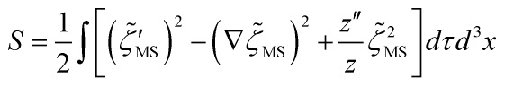
First, let me list the similarities and differences between the single-field slow-roll inflationary scenario and the k−inflationary scenario in both Heisenberg and Schrödinger picture. Note that the -redefined gauge invariant scalar perturbations and of k−inflation and slow-roll inflation, respectively, follow the same action given by:
and:
Thus the Schrödinger k−inflationary scenario would be the same as slow-roll inflation: that is, the variable would follow the same functional Schrödinger equation as in:
with a -modification in the frequency as:
![\[{\omega ^2} = c_s^2{k^2} - \frac{{a''}}{a}\]](https://www.georgeshiber.com/wp-content/ql-cache/quicklatex.com-d2819d9fb1a8ee4a2a661a506425f0a5_l3.png "Rendered by QuickLaTeX.com")
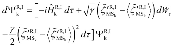
Now, to -modify the k−inflationary scenario with the CSL-collapse dynamics, one just writes the modified Schrödinger picture as such:
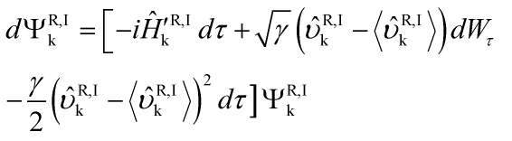
where the wavefunctional  is given by:
![\[\Psi \left[ {\upsilon \left( \tau \right)} \right] = \sum\limits_{\rm{k}} {\Psi _{\rm{k}}^{\rm{R}}} \left[ {\upsilon _{\rm{k}}^{\rm{R}}\left( \tau \right)} \right]\Psi _{\rm{k}}^{\rm{I}}\left[ {\upsilon _{\rm{k}}^{\rm{I}}\left( \tau \right)} \right]\]](https://www.georgeshiber.com/wp-content/ql-cache/quicklatex.com-8669f37dd6067e2d2cb73234cbdcf123_l3.png "Rendered by QuickLaTeX.com")
and the Hamiltonian is:
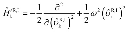
with  defined by:
with equation of motion for  given by:
![\[{\upsilon ''_k} - {\tilde \omega ^2}{\upsilon _k} = 0\]](https://www.georgeshiber.com/wp-content/ql-cache/quicklatex.com-7f0b5a1682073fc8a980f337aaa3734f_l3.png "Rendered by QuickLaTeX.com")
where:
![\[\tilde \omega \equiv {\omega ^3} - 2i\gamma = c_s^2{k^2} - a''/a - 2i\gamma \]](https://www.georgeshiber.com/wp-content/ql-cache/quicklatex.com-7ebf78f07271758eee7cd92c950816e1_l3.png "Rendered by QuickLaTeX.com")
As in the slow-roll inflationary scenario, we fixed the collapse parameter in such a way that it incorporates the amplification mechanism of CSL-dynamics, and the scalar modes in the k−inflationary model travel with a speed  and crosses the sound horizon when .
Hence, the form of the collapse parameter for scalar modes generated during k−inflation is:
![\[\gamma = \frac{{{\gamma _0}\left( k \right)}}{{{{\left( { - {c_s}k\tau } \right)}^\alpha }}}\]](https://www.georgeshiber.com/wp-content/ql-cache/quicklatex.com-3a525a39f2e3f409298a3a06a9182cbc_l3.png "Rendered by QuickLaTeX.com")
Hence it follows that:
![\[{\mathop{\rm Re}\nolimits} {\Omega _k} = \frac{k}{2}{\left( { - k\tau } \right)^{1 - \alpha }}\left( {\frac{{2{\gamma _0}\left( k \right)}}{{c_s^\alpha {k^2}}}} \right)\]](https://www.georgeshiber.com/wp-content/ql-cache/quicklatex.com-2cbdcf26e40fdf2e2e23268605cfb8c8_l3.png "Rendered by QuickLaTeX.com")
which entails that for the parameter range  , the scalar modes in k−inflation becomes classical upon crossing the sound horizon coupled to the inflaton field. Now, the comoving curvature power spectrum on superhorizon scales in k−inflationary scenario, as dictated by:
since we have:
![\[{\mathop{\rm Re}\nolimits} {\Omega _k} = 1/\left( {2{{\left| {{\upsilon _k}} \right|}^2}} \right)\]](https://www.georgeshiber.com/wp-content/ql-cache/quicklatex.com-db9ce3c9baef1d70fd0966605a358cb3_l3.png "Rendered by QuickLaTeX.com")
given by:
![\[{P_R} = \frac{{{k^3}}}{{2{\pi ^2}{z^2}}}{\left| {{\upsilon _k}} \right|^2} = \frac{{{k^3}}}{{4{\pi ^2}{z^2}{\mathop{\rm Re}\nolimits} {\Omega _k}}}\]](https://www.georgeshiber.com/wp-content/ql-cache/quicklatex.com-153066e334b559503d687d435d3ee1e9_l3.png "Rendered by QuickLaTeX.com")
and since  holds, the power spectrum is:
![\[{P_R} = \frac{{{k^2}c_s^{\alpha + 2}{H^2}}}{{8{\pi ^2}{\varepsilon _0}M_{{\rm{PI}}}^2{\gamma _0}\left( k \right)}}{\left( { - k\tau } \right)^{1 + \alpha }}\]](https://www.georgeshiber.com/wp-content/ql-cache/quicklatex.com-af17d566bf49796308bfbbcd83ec9aa3_l3.png "Rendered by QuickLaTeX.com")
and is a function of time and scale . Ridding ourselves from time-dependence, note that:
![\[ - k\tau = \frac{k}{{{k_0}}}{e^{ - \Delta N}}\]](https://www.georgeshiber.com/wp-content/ql-cache/quicklatex.com-d2e8046c5f8ca37a3e6fdc97b6c7d18a_l3.png "Rendered by QuickLaTeX.com")
with the comoving wavenumber of the horizon-mode, thus yielding the form of the comoving curvature power spectrum at the end of inflation as such:
![\[\begin{array}{c}{P_R} = \frac{{k_0^2c_s^{\alpha + 2}{H^2}}}{{8{\pi ^2}{\varepsilon _0}M_{{\rm{PI}}}^2{{\tilde \gamma }_0}}}{\left( {\frac{k}{{{k_0}}}} \right)^{3 + \alpha - \beta }}\\{e^{ - \left( {1 + \alpha } \right)\Delta N}}\end{array}\]](https://www.georgeshiber.com/wp-content/ql-cache/quicklatex.com-d5262afd0f4a57eb388c3dbd9a4ec94e_l3.png "Rendered by QuickLaTeX.com")
giving us a scale-independent spectrum. We can now determine the scalar spectral index as:
![\[{n_s} - 1 = \delta - 2{\varepsilon _0} - {\varepsilon _1} + \left( {\alpha + 2} \right){s_0}\]](https://www.georgeshiber.com/wp-content/ql-cache/quicklatex.com-9355310a30737a7fb6ed3ad72e65cf86_l3.png "Rendered by QuickLaTeX.com")
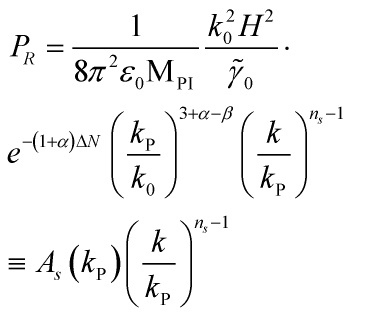
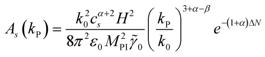
Hence, the comoving curvature power spectrum can be derived as such:
![\[{P_R} \equiv {A_s}\left( {{k_{\rm{P}}}} \right){\left( {\frac{k}{{{k_{\rm{P}}}}}} \right)^{{n_s} - 1}}\]](https://www.georgeshiber.com/wp-content/ql-cache/quicklatex.com-1ea5cff0a81a41f534fe92e9557ace7e_l3.png "Rendered by QuickLaTeX.com")
with  the inflaton-field-pivot scale and the amplitude of the scalar spectrum
  is:
is:
![\[\begin{array}{c}{A_s}\left( {{k_{\rm{P}}}} \right) = \frac{{k_0^2c_s^{\alpha + 2}{H^2}}}{{8{\pi ^2}{\varepsilon _0}M_{{\rm{PI}}}^2}}{\left( {\frac{{{k_{\rm{P}}}}}{{{k_0}}}} \right)^{3 + \alpha - \beta }}\\{e^{ - \left( {1 + \alpha } \right)\Delta N}}\end{array}\]](https://www.georgeshiber.com/wp-content/ql-cache/quicklatex.com-71a8b1e7519cb515ad95e8fb4f284322_l3.png "Rendered by QuickLaTeX.com")
So, tensorial perturbation analysis in k−inflation is equivalent to slow-roll inflation, hence, we can apply CSL-collapse dynamics to tensor modes in k−inflation by use of the collapse parameter form of as given by:
Now we can solve the equation for as given by:
which entails:
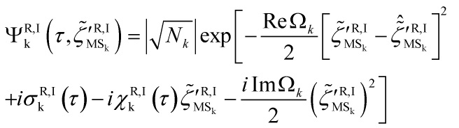
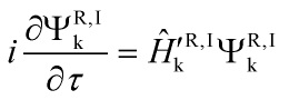
Therefore, CSL-collapse dynamics can explain the primordial cosmological quantum-to-classical phase-transition since the modified Schrödinger equation:
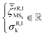
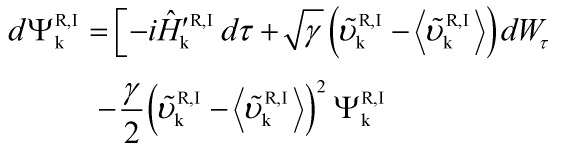 with the wavefuctional given by:
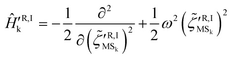
with the Hamiltonian:
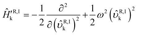
with given by:
So we get the equation of motion for as:
with the crucial identity:
![\[{\tilde \omega ^2} \equiv {\omega ^2} - 2i\gamma = c_s^2{k^2} - a''/a - 2i\gamma \]](https://www.georgeshiber.com/wp-content/ql-cache/quicklatex.com-ffc1fc5927f419c4d01fd49a188cfbdb_l3.png "Rendered by QuickLaTeX.com")
Hence, the collapse parameter for scalar modes generated during k−inflation is:
with  , so we can derive:
entailing that the scalar modes in k−inflation become classical upon crossing the sound horizon during inflation
and the comoving curvature power spectrum on superhorizon-scales in k−inflationary scenario are:
yielding the power spectrum:
Again dependent on time and scale, and to eliminate it, first note that:
with the comoving wavenumber of the mode which is at the present-horizon consistent with CMBR data. So we get the following form of the comoving curvature power spectrum at the end of inflation:
Giving us a scale-independent spectrum with scalar spectral index:
thus reducing the comoving curvature power spectrum to the following form:
![\[{P_R} = {A_s}\left( {{k_{\rm{P}}}} \right){\left( {\frac{k}{{{k_{\rm{P}}}}}} \right)^{{n_s} - 1}}\]](https://www.georgeshiber.com/wp-content/ql-cache/quicklatex.com-6f00c9fdeac24b4036467bc2212f2d56_l3.png "Rendered by QuickLaTeX.com")
with the pivot scale and the amplitude of the scalar spectrum is:
Hence, the tensor perturbation analysis in k−inflation is equivalent to that of the slow-roll inflationary cosmological model, and applying the CSL-collapse dynamics to the tensor modes in k−inflation, we use as defined by:
![\[\gamma : = \frac{{{\gamma _0}\left( k \right)}}{{{{\left( { - k\tau } \right)}^\alpha }}}\]](https://www.georgeshiber.com/wp-content/ql-cache/quicklatex.com-ce2d31e04641f36c69c206b5cc030dfe_l3.png "Rendered by QuickLaTeX.com")
and that yields the same tensor power spectrum and tensor spectral index as given by:
and:
respectively. Thus giving us the tensor-to-scalar ratio:
![\[r = 16{\varepsilon _0}c_s^{ - \left( {\alpha + 2} \right)} = - 8\left( {{n_T} - \delta } \right)c_s^{ - \left( {\alpha + 2} \right)}\]](https://www.georgeshiber.com/wp-content/ql-cache/quicklatex.com-7dced7296e67ba7b9830d0a3ed75e9e3_l3.png "Rendered by QuickLaTeX.com")
Therefore, CSL-collapse dynamics yields a the required neccessary and sufficient consistency condition for k−inflation and drive the quantum-to-classical transition of primordial quantum perturbations generated during the inflationary phase, up to a phase-transition scale factor, feats that both, quantum-Decoherence and Bohmian mechanics fail to resolve or explain.