Continuing from my last post where I discussed the triangular interplay between string-string duality, string field theory, and the action of Dp/M5-branes, here I shall discuss Stueckelberg string fields and derive the BRST invariance of the Landau-Stueckelberg action. Recalling that the action of M-theory in the Witten gauge is:
![\[\begin{array}{l}{S_M} = \frac{1}{{{k^9}}}\int\limits_{{\rm{world - volumes}}} {{d^{11}}} \sqrt {\frac{{ - {g_{\mu \nu }}}}{{ - \gamma }}} {T_p}^{10}d\Omega {\left( {{\phi _{INST}}} \right)^{26}}\left( {{R_{icci}} - A_\mu ^H\frac{1}{{48}}G_4^2} \right) + \\\sum\limits_{Dp} {D_\mu ^{SuSy}} {e^{ - H_3^b}}/S_{Dp}^{WV} + \sum\limits_{Dp} {D_\nu ^{SuSy}} {e^{H_3^b}}/S_{Dp}^{SV}\end{array}\]](https://www.georgeshiber.com/wp-content/ql-cache/quicklatex.com-1a699b31134d813b59d880d2e5f88662_l3.png "Rendered by QuickLaTeX.com")
with  the kappa symmetry term,
  the metric on
  , and
, and  the corresponding coordinates with
  an antisymmetric 3-tensor. Hence, the worldvolume
  is:
is:
![\[R \times {S^1} \times {S^1}/{Z_2}\]](https://www.georgeshiber.com/wp-content/ql-cache/quicklatex.com-32cbccc7e51757f72dc1fbc5b9e2a973_l3.png "Rendered by QuickLaTeX.com")
and the worldsheet action:
![\[{S_{het}} = {S_{st}} + {S_{KK}} + {S_{\bmod }}\]](https://www.georgeshiber.com/wp-content/ql-cache/quicklatex.com-81a754148a2c99518936ae3ed71b4a5e_l3.png "Rendered by QuickLaTeX.com")
being the sum of three terms:
![\[{S_{st}} = \int {{d^2}} \sigma \frac{1}{2}\left( {{g_{mn}}{\eta ^{ij}} + {b_{mn}}{\varepsilon ^{ij}}} \right){\partial _i}{x^m}{\partial _j}{x^n}\]](https://www.georgeshiber.com/wp-content/ql-cache/quicklatex.com-0629b1e6eedba3792e43442cb7c8f36c_l3.png "Rendered by QuickLaTeX.com")
![\[{S_{KK}}\int {{d^2}} \sigma {\varepsilon ^{ij}}{\partial _i}{x^I}{\partial _j}{x^m}A_m^I\]](https://www.georgeshiber.com/wp-content/ql-cache/quicklatex.com-321bba037609cead48bbf2d93b34bd6d_l3.png "Rendered by QuickLaTeX.com")
![\[{S_{\,\bmod \,}} = \int {{d^2}} \sigma \frac{1}{2}\left( {{g_{IJ}}{\eta ^{ij}} + {b_{IJ}}{\varepsilon ^{ij}}} \right){\partial _i}{x^J}{\partial _j}{x^I}\]](https://www.georgeshiber.com/wp-content/ql-cache/quicklatex.com-60cffd8d87242328b3552e5b5f9d9b34_l3.png "Rendered by QuickLaTeX.com")
and the index I = 1, … , 22 labels 22 gauge fields: 16 coming from the internal dimensions of the heterotic string, and the other 6 gauge fields are the KK modes of the metric and antisymmetric tensor. The action  has a massless spectrum given by moduli fields corresponding to deformations of the Narain lattice and thus take values in the group manifold:
![\[\frac{{SO\left( {19,3} \right)}}{{SO\left( {19} \right) \times SO\left( 3 \right)}}\]](https://www.georgeshiber.com/wp-content/ql-cache/quicklatex.com-36acfc52490cab43de512dee7ad8cb13_l3.png "Rendered by QuickLaTeX.com")
Something deep has occurred: all the gauge fields of the action  have appeared within a two-dimensional theory, and not a three-dimensional theory
have appeared within a two-dimensional theory, and not a three-dimensional theorywhich is precisely the long wavelength limit behavior of the open membrane:
the gauge fields are defined in terms of fields that live on 10-dimensional boundaries of M-theory
In the closed membrane case:
the gauge fields are defined in terms of 11-dimensional fields
which brought us to the connection between string field theory and Dp-branes. Recall that one derives the string propagator by an evaluation of the Witten super-symmetric quantum path integral on a fiber-strip with the Polyakov string action:
![\[G\left[ {{X_1};{X_2}} \right] = \int {D\left[ h \right]} D\left[ X \right]\exp \left( {iS} \right)\]](https://www.georgeshiber.com/wp-content/ql-cache/quicklatex.com-798fe18248f6089fbf239f15e3dd158c_l3.png "Rendered by QuickLaTeX.com")
with:
![\[S = - \frac{1}{{4\pi \alpha '}}\int_M {d\tau d\sigma } \sqrt { - h} {h^{\alpha \beta }}\frac{{\partial {X^I}}}{{\partial {\sigma ^\alpha }}}\frac{{\partial {X^J}}}{{\partial {\sigma ^\beta }}}{\eta _{IJ}}\]](https://www.georgeshiber.com/wp-content/ql-cache/quicklatex.com-da305c8be1d257dd1323751682e03cd3_l3.png "Rendered by QuickLaTeX.com")
for  and the Regge parameter clear from context. In the proper-time gauge and the normal modes of the lapse and shift function in 2-D, the Polyakov metric has the following property:
![\[\sqrt { - h} {h^{\alpha \beta }} = \frac{1}{{{N_1}}}\left( {\begin{array}{*{20}{c}}{ - 1}&{{N_2}}\\{{N_2}}&{{{\left( {{N_1}} \right)}^2} - {{\left( {{N_2}} \right)}^2}}\end{array}} \right)\]](https://www.georgeshiber.com/wp-content/ql-cache/quicklatex.com-9ae8c45d036885c10dc38e6ff59b5dbd_l3.png "Rendered by QuickLaTeX.com")
allowing us to derive the open string field Polyakov propagator on the Dp-branes:
![\[\begin{array}{c}G\left[ {{X_1};{X_2}} \right) = \int_0^\infty {ds} \left\langle {{X_1}\left| {\exp \left[ { - is\left( {{L_0} - i\tilde \varepsilon } \right)} \right]} \right|{X_2}} \right\rangle \\ = \left\langle {{X_1}\left| {\frac{1}{{{L_0} - i\tilde \varepsilon }}} \right|{X_2}} \right\rangle \end{array}\]](https://www.georgeshiber.com/wp-content/ql-cache/quicklatex.com-89438f647f490708cfa6e25a36fb1a7c_l3.png "Rendered by QuickLaTeX.com")
with:
![\[{L_0} = \frac{{{p^\mu }{p_\mu }}}{2} + \sum\limits_{n = 1} {\frac{1}{2}} \left( {p_n^Ip_n^J + {n^2}x_n^Ix_n^J} \right){\eta _{IJ}} - 1\]](https://www.georgeshiber.com/wp-content/ql-cache/quicklatex.com-6d60fddf6bf43dec74fc87fd21577875_l3.png "Rendered by QuickLaTeX.com")
and the momentum operators are given by:
![\[{P^\mu }\left( \sigma \right) = \frac{1}{\pi }{\left( {{p^\mu } + \sqrt 2 \sum\limits_{n = 1} {p_n^\mu \cos \left( {n\sigma } \right)} } \right)_{,\mu = 0,1,...,d}}\]](https://www.georgeshiber.com/wp-content/ql-cache/quicklatex.com-19aa95d541a432d36912934ee4da0545_l3.png "Rendered by QuickLaTeX.com")
![\[{P^i}\left( \sigma \right) = \frac{{\sqrt 2 }}{\pi }{\sum\limits_{n = 1} {p_n^i\sin \left( {n\sigma } \right)} _{,i = 0,1,...,d}}\]](https://www.georgeshiber.com/wp-content/ql-cache/quicklatex.com-8e20579a7449b7d5bdbff4e53754b083_l3.png "Rendered by QuickLaTeX.com")
Since open string end-points are topologically glued to  Dp-branes, open strings must have
  inequivalent quantum states and thus, the string field
  has to carry the gauge group indices of
  :
:
![\[\Psi \left[ X \right] = \frac{1}{{\sqrt 2 }}{\Psi ^0}\left[ X \right] + {\Psi ^a}\left[ X \right]{T^a}\]](https://www.georgeshiber.com/wp-content/ql-cache/quicklatex.com-c5e27c084525d92f86754729a2d582fc_l3.png "Rendered by QuickLaTeX.com")
where  are the generators of the SU(N) group, with
  . Hence, the string propagator on multi-Dp-branes takes the following form, with contraction and indices ordering:
![\[\begin{array}{l}{G^{ab}}\left[ {{X_1};{X_2}} \right] = i\left\langle {T{\Psi ^a}\left[ {{X_1}} \right]{\Psi ^b}\left[ {{X_2}} \right]} \right\rangle \\ = i\int D \left[ X \right]{\Psi ^a}\left[ {{X_1}} \right]{\Psi ^b}\left[ {{X_2}} \right]\exp \left\{ { - i\int {D\left[ X \right]{\rm{tr}}\Psi \left( {{L_0} + i\tilde \varepsilon } \right)\Psi } } \right\}\end{array}\]](https://www.georgeshiber.com/wp-content/ql-cache/quicklatex.com-bc885ff62f8a5f00226a13c4b93595b2_l3.png "Rendered by QuickLaTeX.com")
which yields the field theory action:
![\[{S_0} = \int {D\left[ X \right]} {\rm{tr}}\Psi \left( {{L_0} - i\tilde \varepsilon } \right)\Psi \]](https://www.georgeshiber.com/wp-content/ql-cache/quicklatex.com-32774ac27766b67c2424ab329e11df4d_l3.png "Rendered by QuickLaTeX.com")
BRST-invariantly as:
![\[{S_0} = \int {{\rm{tr}}\Psi } * Q_{BRST}^{generators}\Psi \]](https://www.georgeshiber.com/wp-content/ql-cache/quicklatex.com-9b3038c73f91afcf152347a5be6cd8af_l3.png "Rendered by QuickLaTeX.com")
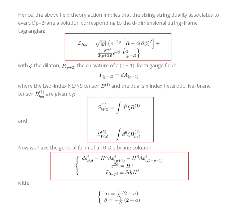
Hence, the above field theory action implies that the string-string duality associates to every Dp–Brane a solution corresponding to the d–dimensional string–frame Lagrangian:
![\[\begin{array}{c}{\mathcal{L}_{S,d}} = \sqrt {\left| g \right|} \left\{ {{e^{ - 2\phi }}} \right.\left[ {R - 4{{\left( {\partial \phi } \right)}^2}} \right] + \\\frac{{{{( - )}^{p + 1}}}}{{2\left( {p + 2} \right)!}}{e^{a\phi }}\left. {F_{\left( {p + 2} \right)}^2} \right\}\end{array}\]](https://www.georgeshiber.com/wp-content/ql-cache/quicklatex.com-e595d8bd49324003a7101ba1a1a1a8fb_l3.png "Rendered by QuickLaTeX.com")
with  the dilaton,
  the curvature of a (p + 1)–form gauge field:
![\[{F_{\left( {p + 2} \right)}} = d{A_{\left( {p + 1} \right)}}\]](https://www.georgeshiber.com/wp-content/ql-cache/quicklatex.com-cd0c901de42bb6693fe2801fd4a9f2b0_l3.png "Rendered by QuickLaTeX.com")
where the two–index NS/NS tensor  and the dual six-index heterotic five–brane tensor
  are given by:
![\[S_{WZ}^{(1)} = \int {{d^2}} \xi {B^{(1)}}\]](https://www.georgeshiber.com/wp-content/ql-cache/quicklatex.com-5d8b9edae194db0d7a556ece4fa9f6c1_l3.png "Rendered by QuickLaTeX.com")
and
![\[S_{WZ}^{(5)} = \int {{d^6}} \xi \tilde B_{het}^{(1)}\]](https://www.georgeshiber.com/wp-content/ql-cache/quicklatex.com-5b105c67ef55e788a6d680ffdcb1aa0f_l3.png "Rendered by QuickLaTeX.com")
Now we have the general form of a 10-D p-brane solution:
![\[\left\{ {\begin{array}{*{20}{c}}{ds_{S,d}^2 = {H^\alpha }dx_{\left( {p + 1} \right)}^2 - {H^\beta }dx_{\left( {D - p - 1} \right)}^2}\\{{e^{2\phi }} = {H^\gamma }}\\{{F_{0...pi}} = \delta {\partial _i}{H^{\tilde \varepsilon }}}\end{array}} \right.\]](https://www.georgeshiber.com/wp-content/ql-cache/quicklatex.com-2289bec5801dc6befb29272db1a7515b_l3.png "Rendered by QuickLaTeX.com")
with:
![\[\left\{ {\begin{array}{*{20}{c}}{\alpha = \frac{1}{N}\left( {2 - a} \right)}\\{\beta = - \frac{1}{N}\left( {2 + a} \right)}\end{array}} \right.\]](https://www.georgeshiber.com/wp-content/ql-cache/quicklatex.com-b182b607ad4469d90d42c16b510ad6b1_l3.png "Rendered by QuickLaTeX.com")
and:
![\[\left\{ {\begin{array}{*{20}{c}}{\gamma = \frac{1}{N}\left[ {2\left( {p + 1} \right) + \left( {2 + a} \right)\left( {1 - \frac{1}{2}d} \right)} \right]}\\{{\delta ^2} = - \frac{4}{N},\quad \,\tilde \varepsilon = - 1}\end{array}} \right.\]](https://www.georgeshiber.com/wp-content/ql-cache/quicklatex.com-a044702ce4ba6147ef16eec78b0e1c34_l3.png "Rendered by QuickLaTeX.com")
with
![\[N = \left( {p + 1} \right)a + \left( {1 - \frac{1}{2}d} \right){\left( {1 + \frac{1}{2}a} \right)^2}\]](https://www.georgeshiber.com/wp-content/ql-cache/quicklatex.com-67348340f5803c0b582c76ab4e083b0c_l3.png "Rendered by QuickLaTeX.com")
The general form of 11-D Mp–branes solutions, noting the absence of the dilaton field, with the following Lagrangian:
![\[{\mathcal{L}_{Ein,d}} = \sqrt {\left| g \right|} \left[ {R + \frac{1}{2}{{\left( {\partial \phi } \right)}^2} + \frac{{{{( - )}^{p + 1}}}}{{2\left( {p + 2} \right)!}}{e^{\alpha \phi }}F_{\left( {p + 2} \right)}^2} \right]\]](https://www.georgeshiber.com/wp-content/ql-cache/quicklatex.com-66fe4e93349a0e2c7ade0c36f5b8fb86_l3.png "Rendered by QuickLaTeX.com")
is:
![\[\begin{array}{*{20}{c}}{\alpha = - \frac{4}{N}\left( {d - p - 3} \right),}&{\beta = \frac{4}{N}\left( {p + 1} \right)}\\{\gamma = \frac{{4a}}{N}\left( {d - 2} \right),}&\begin{array}{l}{\delta ^2} = \frac{4}{N}\left( {d - 2} \right)\\\tilde \varepsilon = - 1\end{array}\end{array}\]](https://www.georgeshiber.com/wp-content/ql-cache/quicklatex.com-5a39bda56f1832e2848d86fd66141721_l3.png "Rendered by QuickLaTeX.com")
Hence, the M2-brane solution is:
![\[ds_{Ein,11}^2 = {H^{ - 2/3}}dx_{\left( 3 \right)}^2 - {H^{1/3}}dx_{\left( 8 \right)}^2\]](https://www.georgeshiber.com/wp-content/ql-cache/quicklatex.com-af2a8ff75cc6f20b3bfa0966dbfe56bd_l3.png "Rendered by QuickLaTeX.com")
![\[{F_{012i}} = {\partial _i}{H^{ - 1}}\]](https://www.georgeshiber.com/wp-content/ql-cache/quicklatex.com-4f548887d4bdcec24b1a5cb6c62b8002_l3.png "Rendered by QuickLaTeX.com")
squaring the field strength gives the following M5-brane solution:
![\[ds_{Ein,11}^2 = {H^{ - 1/3}}dx_{\left( 6 \right)}^2 - {H^{2/3}}dx_{\left( 5 \right)}^2\]](https://www.georgeshiber.com/wp-content/ql-cache/quicklatex.com-ad2906fb1b75064bea61b2a955c2a32f_l3.png "Rendered by QuickLaTeX.com")
![\[{F_{012345i}} = {\partial _i}{H^{ - 1}}\]](https://www.georgeshiber.com/wp-content/ql-cache/quicklatex.com-347ea734ef507639f370b94b3e6ed855_l3.png "Rendered by QuickLaTeX.com")
In the string-frame Ramond-Ramond gauge field Lagrangian:
Dp-brane solutions have the following form:
![\[ds_{S,10}^2 = {H^{ - 1/2}}dx_{\left( {p + 1} \right)}^2 - {H^{1/2}}dx_{\left( {9 - p} \right)}^2\]](https://www.georgeshiber.com/wp-content/ql-cache/quicklatex.com-04f51d7d8c33db506ee2eec2b1336ec0_l3.png "Rendered by QuickLaTeX.com")
![\[{e^{2\phi }} = {H^{ - \frac{1}{2}\left( {p - 3} \right)}}\]](https://www.georgeshiber.com/wp-content/ql-cache/quicklatex.com-1f830668c0ea714c70b54e0b881afe1d_l3.png "Rendered by QuickLaTeX.com")
![\[{F_{0...pi}} = {\partial _i}{H^{ - 1}}\]](https://www.georgeshiber.com/wp-content/ql-cache/quicklatex.com-45311ed56ba79961d8f7751080d9815d_l3.png "Rendered by QuickLaTeX.com")
From the string-string duality above and  , we can derive the kinetic term of Dp–branes in terms of the Born–Infeld action with the following form:
![\[{S^{Dp}} = \int {{d^{p + 1}}} \xi {e^{ - \phi }}\sqrt {\left| {\det \left( {{g_{ij}} + {{\tilde F}_{ij}}} \right)} \right|} \]](https://www.georgeshiber.com/wp-content/ql-cache/quicklatex.com-5da9298ee92a4d6d6a2f89ce2bf9f8be_l3.png "Rendered by QuickLaTeX.com")
with the embedding metric and the gauge field world-volume curvature manifest, entailing the existence of a WZ/RR term that couples to Dp-branes:
![\[S_{WZ}^{Dp} = \int {{d^{p + 1}}} \xi \tilde {\rm A}{e^{\tilde F}}\]](https://www.georgeshiber.com/wp-content/ql-cache/quicklatex.com-e66428719be07e30dd2fdaad3d39a249_l3.png "Rendered by QuickLaTeX.com")
![\[\tilde {\rm A} = \sum\nolimits_{q = 0}^9 {{A_{\left( {q + 1} \right)}}} \]](https://www.georgeshiber.com/wp-content/ql-cache/quicklatex.com-676b3af87cdd0048fa2e637b7f334ea8_l3.png "Rendered by QuickLaTeX.com")
and where the heterotic 5–brane, the IIA five–brane and the D5–brane dual potentials are given by:
![\[^ * d{B^{(1)}} = d\tilde B_{het}^{(1)}\]](https://www.georgeshiber.com/wp-content/ql-cache/quicklatex.com-fe6867b4ded1eccac69412545aa940fe_l3.png "Rendered by QuickLaTeX.com")
![\[^ * d{B^{(1)}} = d\tilde B_{{\rm{IIA}}}^{(1)} - \frac{{105}}{4}CdC - 7{A^{(1)}}G\left( {\tilde C} \right)\]](https://www.georgeshiber.com/wp-content/ql-cache/quicklatex.com-85380d11cc934d49ceb6f63f0c8cfc4d_l3.png "Rendered by QuickLaTeX.com")
![\[^ * d{B^{(1)}} = d\tilde B_{{\rm{IIB}}}^{(1)} + Dd{B^{(2)}} - \frac{1}{4}{{\tilde \varepsilon }^{kl}}{B^{(2)}}{B^{(k)}}d{B^{(1)}}\]](https://www.georgeshiber.com/wp-content/ql-cache/quicklatex.com-f32f16edeb5c35829783b38c0fcde67a_l3.png "Rendered by QuickLaTeX.com")
Parallels for the M5-brane are formally similar. We have the quadratic kinetic term:
![\[{S^{M5}} = \int {{d^6}} \xi \sqrt {\left| g \right|} \left[ {1 + \frac{1}{2}{\mathcal{H}^2} + \wp \left( {{\mathcal{H}^4}} \right)} \right]\]](https://www.georgeshiber.com/wp-content/ql-cache/quicklatex.com-86f210b320ac013424507390120f5110_l3.png "Rendered by QuickLaTeX.com")
with the WZ term:
![\[S_{WZ}^{M5} = \int {{d^6}} \xi \left[ {\frac{1}{{70}}\tilde C + \frac{3}{4}\mathcal{H}C} \right]\]](https://www.georgeshiber.com/wp-content/ql-cache/quicklatex.com-8ac461ac558e4ebab8f2b83e7e9f9956_l3.png "Rendered by QuickLaTeX.com")
and the dual 6–form potential:
![\[d\tilde C - \frac{{105}}{4}CdC = {\,^ * }dC\]](https://www.georgeshiber.com/wp-content/ql-cache/quicklatex.com-9fdd82d658a85a53878cbc0e9f05a717_l3.png "Rendered by QuickLaTeX.com")
By the field-property of the Polyakov propagator on the Dp-branes:
combined with the string-string duality, we can prove that all Dp-and-Mn–brane solutions preserve half of the SUSY. With the SUSY rules for the gravitino and dilatino in the string-frame given by:
![\[\delta {\psi _\mu } = {\partial _\mu }\tilde \varepsilon - \frac{1}{4}{\omega _\mu }^{ab}{\gamma _{ab}}\tilde \varepsilon + \frac{{{{( - )}^p}}}{{8\left( {p + 2} \right)!}}{e^\phi }F \cdot \gamma {\gamma _\mu }{{\tilde \varepsilon '}_{(p)}}\]](https://www.georgeshiber.com/wp-content/ql-cache/quicklatex.com-581ce470af8f9c4fb35d2d23a893d526_l3.png "Rendered by QuickLaTeX.com")
![\[\delta \lambda = {\gamma ^\mu }\left( {{\partial _\mu }\phi } \right)\tilde \varepsilon + \frac{{3 - p}}{{4\left( {p + 2} \right)!}}{e^\phi }F \cdot {\gamma _\mu }{{\tilde \varepsilon '}_{(p)}}\]](https://www.georgeshiber.com/wp-content/ql-cache/quicklatex.com-d1333615d66a38efc787410de8a91192_l3.png "Rendered by QuickLaTeX.com")
![\[F \cdot \gamma \equiv {F_{{\mu _1},,,{\mu _{p + 2}}}}{\gamma ^{{\mu _1},,,{\mu _{p + 2}}}}\]](https://www.georgeshiber.com/wp-content/ql-cache/quicklatex.com-ac3c35d634d5ee35929186daef61491d_l3.png "Rendered by QuickLaTeX.com")
Let us consider the gauge covariantization of the proper-time gauge and the Ramond-Ramond gauge discussed above. The action for the covariant bosonic open string field theory is implicitly defined by the BRST operator  :
:
![\[{Q^c} = - \frac{1}{2}\left\langle {{\Phi _1},Q{\Phi _1}} \right\rangle \]](https://www.georgeshiber.com/wp-content/ql-cache/quicklatex.com-f6c11c8a332c8b23feb7d4c89a751ad3_l3.png "Rendered by QuickLaTeX.com")
with respect to the BPZ conjugation-derived inner product, where the string field has the following Fock space expansion:
![\[{\Phi _1} = {\phi ^{\left( 0 \right)}} + {c_0}{\omega ^{\left( { - 1} \right)}}\]](https://www.georgeshiber.com/wp-content/ql-cache/quicklatex.com-f8deb96e31342ef6c3688f18b68b0a8f_l3.png "Rendered by QuickLaTeX.com")
where the following holds:
![\[{\phi ^{\left( 0 \right)}} = \int {\frac{{{d^{26}}p}}{{{{\left( {2\pi } \right)}^{26}}}}} \left[ {\sum\limits_{\left| f \right\rangle } {\left| {{f^{\left( 0 \right)}}} \right\rangle } {\mkern 1mu} {\psi _{\left| f \right\rangle }}\left( p \right)} \right]\]](https://www.georgeshiber.com/wp-content/ql-cache/quicklatex.com-cbe85be5d2fb3cc9cdb12969fe500ca4_l3.png "Rendered by QuickLaTeX.com")
![\[{\omega ^{\left( { - 1} \right)}} = \int {\frac{{{d^{26}}p}}{{{{\left( {2\pi } \right)}^{26}}}}} \left[ {\sum\limits_{\left| g \right\rangle } {\left| {{g^{\left( { - 1} \right)}}} \right\rangle } \,{\psi _{\left| g \right\rangle }}\left( p \right)} \right]\]](https://www.georgeshiber.com/wp-content/ql-cache/quicklatex.com-5599feba894a0a063dcb60518287ea32_l3.png "Rendered by QuickLaTeX.com")
for the bosonic case, and:
![\[\left\{ {\begin{array}{*{20}{c}}{{\psi _{\left| f \right\rangle }}\left( p \right)}\\{{\psi _{\left| g \right\rangle }}\left( p \right)}\end{array}} \right.\]](https://www.georgeshiber.com/wp-content/ql-cache/quicklatex.com-09a7a184f341812d8e55ebf98b50090c_l3.png "Rendered by QuickLaTeX.com")
are the associated space-time fields. We can now write the action as:
![\[{S^c} = - \frac{1}{2}\left\langle {\left( {{\phi ^{\left( 0 \right)}} - \frac{1}{{{L_0}}}{{\tilde Q}_\omega }^{\left( { - 1} \right)}} \right),{c_0}L\left( {{\phi ^{\left( 0 \right)}} - \frac{1}{{{L_0}}}{{\tilde Q}_\omega }^{\left( { - 1} \right)}} \right)} \right\rangle \]](https://www.georgeshiber.com/wp-content/ql-cache/quicklatex.com-19841fff6f8622361eed8482fd669396_l3.png "Rendered by QuickLaTeX.com")
and is invariant under the gauge transformation:
![\[\delta {\Phi _1} = Q{\Lambda _0}\]](https://www.georgeshiber.com/wp-content/ql-cache/quicklatex.com-6e1b3c7e01dd1ed8e994a516c12f0fb7_l3.png "Rendered by QuickLaTeX.com")
with the gauge parameter being a Grassmann string field of
![\[{N^g} = 0\]](https://www.georgeshiber.com/wp-content/ql-cache/quicklatex.com-81d6a1d7829aa2198e07bb5ac28661ee_l3.png "Rendered by QuickLaTeX.com")
given as:
![\[{\Lambda _0} = {\lambda ^{\left( { - 1} \right)}} + {c_0}{\rho ^{\left( { - 2} \right)}}\]](https://www.georgeshiber.com/wp-content/ql-cache/quicklatex.com-e5f5736d500dc1814a9d9b3f13cc9cc0_l3.png "Rendered by QuickLaTeX.com")
In terms of  and
and  , the gauge transformation is expressible as:
![\[\delta {\phi ^{\left( 0 \right)}} = \tilde Q{\lambda ^{\left( { - 1} \right)}} + M{\rho ^{\left( { - 2} \right)}}\]](https://www.georgeshiber.com/wp-content/ql-cache/quicklatex.com-5ec048c3c97ec351290385f6f83916f9_l3.png "Rendered by QuickLaTeX.com")
![\[\delta {\omega ^{\left( { - 1} \right)}} = {L_0}{\lambda ^{\left( { - 1} \right)}} - \tilde Q{\rho ^{\left( { - 2} \right)}}\]](https://www.georgeshiber.com/wp-content/ql-cache/quicklatex.com-d7587b7c89c2a81246bbca484be566c3_l3.png "Rendered by QuickLaTeX.com")
It follows then that:
![\[{\zeta ^{\left( { - 1} \right)}} = \tilde Q{\phi ^{\left( 0 \right)}} + M{\omega ^{\left( { - 1} \right)}}\]](https://www.georgeshiber.com/wp-content/ql-cache/quicklatex.com-a6c3da85471e14695948ac51515300d0_l3.png "Rendered by QuickLaTeX.com")
is gauge invariant. Hence, in terms of  , the action:
becomes:
![\[\begin{array}{c}{S^c} = - \frac{1}{2}\left( {\left\langle {{\phi ^{\left( 0 \right)}},{c_0}{L_0}{\phi ^{\left( 0 \right)}}} \right\rangle - \left\langle {\tilde Q{\phi ^{\left( 0 \right)}},{c_0}{W_1}\left( {\tilde Q{\phi ^{\left( 0 \right)}}} \right)} \right\rangle } \right.\\ + \left. {\left\langle {{\zeta ^{\left( 1 \right)}},{c_0}{W_1}{\zeta ^{\left( 1 \right)}}} \right\rangle } \right)\end{array}\]](https://www.georgeshiber.com/wp-content/ql-cache/quicklatex.com-459699a274d6c23adea1710a8f600648_l3.png "Rendered by QuickLaTeX.com")
Note that the gauge invariance of each of:
![\[{\left\langle {{\zeta ^{\left( 1 \right)}},{c_0}{W_1}{\zeta ^{\left( 1 \right)}}} \right\rangle }\]](https://www.georgeshiber.com/wp-content/ql-cache/quicklatex.com-562da7f5ca6c6c82459287c5bfb032d9_l3.png "Rendered by QuickLaTeX.com")
and
![\[{\left\langle {{\phi ^{\left( 0 \right)}},{c_0}{L_0}{\phi ^{\left( 0 \right)}}} \right\rangle - \left\langle {\tilde Q{\phi ^{\left( 0 \right)}},{c_0}{W_1}\left( {\tilde Q{\phi ^{\left( 0 \right)}}} \right)} \right\rangle }\]](https://www.georgeshiber.com/wp-content/ql-cache/quicklatex.com-e4e2fffeb6c7ee5ad76976be4fdb0cd2_l3.png "Rendered by QuickLaTeX.com")
entails that the string field, by conformal gauge theory, has the following form:
![\[\phi _{N \le 1}^{\left( 0 \right)} = \int {\frac{{{d^{26}}p}}{{{{\left( {2\pi } \right)}^{26}}}}} \frac{1}{{\sqrt {\alpha '} }}\left( {\phi \left( p \right)\left| {0,p; \downarrow } \right\rangle + {A_\mu }\left( p \right)\alpha _{ - 1}^\mu \left| {0,p, \downarrow } \right\rangle } \right)\]](https://www.georgeshiber.com/wp-content/ql-cache/quicklatex.com-9713c58326dbfa420b7a886da007a1eb_l3.png "Rendered by QuickLaTeX.com")
![\[\omega _{N \le 1}^{\left( 0 \right)} = \int {\frac{{{d^{26}}p}}{{{{\left( {2\pi } \right)}^{26}}}}} \frac{i}{{\sqrt 2 }}\chi \left( p \right){b_{ - 1}}\left| {0,p; \downarrow } \right\rangle \]](https://www.georgeshiber.com/wp-content/ql-cache/quicklatex.com-9bb667b39c923a23f47e239b7cd0f26d_l3.png "Rendered by QuickLaTeX.com")
and we also have:
![\[\zeta _{N \le 1}^{\left( 1 \right)} = \int {\frac{{{d^{26}}p}}{{{{\left( {2\pi } \right)}^{26}}}}} \sqrt 2 \left( { - i\chi \left( p \right) + {A_\mu }\left( p \right){p^\mu }} \right){c_{ - 1}}\left| {0,p; \downarrow } \right\rangle \]](https://www.georgeshiber.com/wp-content/ql-cache/quicklatex.com-7acc20fbf0613e634023d4e9cf218dfd_l3.png "Rendered by QuickLaTeX.com")
Thus, our action becomes a sum of two gauge invariant terms:
![\[ - \frac{1}{2}\left( {\left\langle {{\phi ^{\left( 0 \right)}},{c_0}{L_0}{\phi ^{\left( 0 \right)}}} \right\rangle - \left\langle {\tilde Q{\phi ^{\left( 0 \right)}},{c_0}{W_1}\left( {\tilde Q{\phi ^{\left( 0 \right)}}} \right)} \right\rangle } \right)\left| {_{N \le 1}} \right.\]](https://www.georgeshiber.com/wp-content/ql-cache/quicklatex.com-d6e0268fa5e65df6128acf69722999c5_l3.png "Rendered by QuickLaTeX.com")
and
![\[ - \frac{1}{2}\left\langle {{\zeta ^{\left( 1 \right)}},{c_0}{W_1}{\zeta ^{\left( 1 \right)}}} \right\rangle \left| {_{N \le 1}} \right.\]](https://www.georgeshiber.com/wp-content/ql-cache/quicklatex.com-f0331d5f8ec61d66f0553f9fd6757fc4_l3.png "Rendered by QuickLaTeX.com")
Now, crucially:
![\[{\left\langle {\tilde Q{\phi ^{\left( 0 \right)}},{c_0}{W_1}\left( {\tilde Q{\phi ^{\left( 0 \right)}}} \right)} \right\rangle }\]](https://www.georgeshiber.com/wp-content/ql-cache/quicklatex.com-c06e38d5c0c1539c9b08ac7a12a47819_l3.png "Rendered by QuickLaTeX.com")
is equivalent to a gauge invariant action of massless vector field 
and by the metaplecticity of:
![\[\left\langle {{\zeta ^{\left( 1 \right)}},{c_0}{W_1}{\zeta ^{\left( 1 \right)}}} \right\rangle \]](https://www.georgeshiber.com/wp-content/ql-cache/quicklatex.com-6fea7428175e459b13c67d88d405244b_l3.png "Rendered by QuickLaTeX.com")
it follows that gauge transformation up to level N = 1 is expandible in terms of a gauge parameter  as:
as:
![\[\delta {A_\mu }\left( p \right) = i{p_\mu }\lambda \]](https://www.georgeshiber.com/wp-content/ql-cache/quicklatex.com-78329e5d82bac232ff14797ee24d53b3_l3.png "Rendered by QuickLaTeX.com")
![\[\delta \chi \left( p \right) = {p^2}\lambda \]](https://www.georgeshiber.com/wp-content/ql-cache/quicklatex.com-338f1682f2cc0a8b809599f91f0293cd_l3.png "Rendered by QuickLaTeX.com")
We perform now a Virasoro reparametrization of the evolving string surface as a transformation:
![\[\delta \left| \Phi \right\rangle = i\sum\limits_{n = - \infty }^\infty {{b_n}{L_{ - n}}} \left| \Phi \right\rangle \]](https://www.georgeshiber.com/wp-content/ql-cache/quicklatex.com-2e7d42580f4acd75dafe70dd35fd5b2c_l3.png "Rendered by QuickLaTeX.com")
with 
the wave-function of the string, which in string field theory, must be interpreted as a functional ![\Phi \left[ {x\left( \sigma \right)} \right]](https://www.georgeshiber.com/wp-content/ql-cache/quicklatex.com-33a93e92344c7106acbe82cf55395752_l3.png "Rendered by QuickLaTeX.com") , giving us the functional action:
, giving us the functional action:
![\[{S_R} = - \frac{1}{2}\left\langle {\Phi \left| {\left. {{K_R}\Phi } \right\rangle } \right.} \right.\]](https://www.georgeshiber.com/wp-content/ql-cache/quicklatex.com-b75a0fcb4bcab5d37355fc74c759ae38_l3.png "Rendered by QuickLaTeX.com")
where the inner product is defined in terms of integrals over the whole string configuration space and  the string field kinetic energy operator. By reparametrization invariance, we can derive the following:
![\[\delta {S_R} = - \frac{i}{2}\sum\limits_n {{b_n}} \left( {\Phi \left[ {{K_R},{L_{ - n}}} \right]\Phi } \right)\]](https://www.georgeshiber.com/wp-content/ql-cache/quicklatex.com-4365ca12f0b9ff6c981863af62fe57af_l3.png "Rendered by QuickLaTeX.com")
and the following relations can be easily checked:
![\[{L_n}\Phi \left[ {x\left( \sigma \right)} \right] = {0_{,\quad n\, > 0}}\]](https://www.georgeshiber.com/wp-content/ql-cache/quicklatex.com-67a894d6778332ba6bc625af5783b957_l3.png "Rendered by QuickLaTeX.com")
![\[\left\{ {\begin{array}{*{20}{c}}{\left[ {K,{L_0}} \right] = 0}\\{K{L_{ - n}} = {0_{,\quad n\, > 0}}}\end{array}} \right.\]](https://www.georgeshiber.com/wp-content/ql-cache/quicklatex.com-5b0c6e489024a80c8ce1f1518c137ddb_l3.png "Rendered by QuickLaTeX.com")
Now, what makes unique contrastively to  is its invariance under an large group of extra symmetries in addition to reparametrization implicitly expressed by:
specifically, given by shifts:
![\[\delta \Phi \left[ {x\left( \sigma \right)} \right] = \mathcal{L}_{ - i}^{\left( n \right)}{\Psi _{ni}}\left[ {x\left( \sigma \right)} \right]\]](https://www.georgeshiber.com/wp-content/ql-cache/quicklatex.com-0a5bb7989efb910b8d8f9ae8bc56f019_l3.png "Rendered by QuickLaTeX.com")
and is a type of meta-gauge symmetry acting directly on the metaplectic phase space. Let us study some properties of this metaplectic gauge group as well as .
We expand  in terms of the eigenstates of the mass operator:
![\[2\left( {{L_0} - 1} \right) = {p^2} + 2\left\{ {\sum\limits_{n > 0} {{\alpha _{ - n}}} \cdot {\alpha _n} - 1} \right\} = {p^2} + {M^2}\]](https://www.georgeshiber.com/wp-content/ql-cache/quicklatex.com-97a4777310c0bc325097a34ff09231c5_l3.png "Rendered by QuickLaTeX.com")
where the state  is annihilated by all
  . Then the string field functional can be written as:
![\[\begin{array}{l}\Phi \left[ {x\left( \sigma \right)} \right] = \left\{ {\phi \left( x \right)} \right. - i{A^\mu }\left( x \right)\alpha _{ - 1}^\mu - \\\frac{1}{2}{h^{\mu \nu }}\left( x \right)\alpha _{ - 1}^\mu \alpha _{ - 1}^\nu i{v^\mu }\alpha _{ - 2}^\mu \left. { + ...} \right\}{\Phi ^{\left( 0 \right)}}\end{array}\]](https://www.georgeshiber.com/wp-content/ql-cache/quicklatex.com-1bdd4e6a8e005ed2bb63b92997ec72a7_l3.png "Rendered by QuickLaTeX.com")
The kinetic gauge of is given by the action of  on new string functionals. At first order we get the following equation of motion:
![\[\begin{array}{c}{L_{ - 1}}\Psi \left[ {x\left( \sigma \right)} \right] = \left( {p \cdot {\alpha _{ - 1}} + {\alpha _{ - 2}} \cdot + ...} \right)\left\{ {{\phi _\Psi }\left( x \right) - iA_\Psi ^\mu \left( x \right)\alpha _{ - 1}^\mu + ...} \right\}{\Phi ^{\left( 0 \right)}}\\ = \left\{ { - i{\partial ^\mu }{\phi _\Psi }\left( x \right) \cdot \alpha _{ - 1}^\mu + ...} \right\}{\Phi ^{\left( 0 \right)}}\end{array}\]](https://www.georgeshiber.com/wp-content/ql-cache/quicklatex.com-53db8a1eae3ab4a40181f98d20f361fc_l3.png "Rendered by QuickLaTeX.com")
and since  satisfies:
![\[\delta {A^\mu } = {\partial ^\mu }{\phi _\Psi }\]](https://www.georgeshiber.com/wp-content/ql-cache/quicklatex.com-7ff35202ce55420b2334a30b61fa336e_l3.png "Rendered by QuickLaTeX.com")
it follows that:
has the property of linearized Yang-Mills gauge invariance and the following transformation laws can be derived:
![\[\delta {h^{\mu \nu }} = \left( {{\partial ^\mu }A_\Psi ^\nu + {\partial ^\nu }A_\Psi ^\mu } \right) - {\eta ^{\mu \nu }}{\phi _\Xi }\]](https://www.georgeshiber.com/wp-content/ql-cache/quicklatex.com-6c1ed3d539bb1a5763e837e0a93a0d61_l3.png "Rendered by QuickLaTeX.com")
![\[\delta {v^\mu } = A_\Psi ^\mu + {\partial ^\mu }{\phi _\Xi }\]](https://www.georgeshiber.com/wp-content/ql-cache/quicklatex.com-1cde578c7640027a1a56e79eeed7f270_l3.png "Rendered by QuickLaTeX.com")
where  is the Chan-Paton field term.
With  a 0-level state and an eigenstate of
  with eigenvalue
  , we have the following definition for the contravariant form
![\[M_{ij}^{\left( n \right)}\left( h \right) = \left\langle h \right|\mathcal{L}_i^{\left( n \right)}\mathcal{L}_{ - j}^{\left( n \right)}\left| h \right\rangle \]](https://www.georgeshiber.com/wp-content/ql-cache/quicklatex.com-b79c15fe7652402a27193aa7d831b385_l3.png "Rendered by QuickLaTeX.com")
Now we must define:
![\[{\Pi ^{\left( n \right)}} = 1 - \mathcal{L}_{ - i}^{\left( n \right)}M_{ij}^{\left( n \right) - 1}\left( {{L_0}} \right)\mathcal{L}_j^{\left( n \right)}\]](https://www.georgeshiber.com/wp-content/ql-cache/quicklatex.com-f0b171839dba89adc5c92f7d38f0e6bc_l3.png "Rendered by QuickLaTeX.com")
satisfying:
![\[{\Pi ^{\left( n \right)}} = {\Phi _m} = {\Phi _m}\,\,,\quad m < n\]](https://www.georgeshiber.com/wp-content/ql-cache/quicklatex.com-b87c2f81fcff1ba34c178c9e077dedf3_l3.png "Rendered by QuickLaTeX.com")
![\[{\Pi ^{\left( n \right)}} = {\Phi _n} = {\Pi ^{\left( n \right)}}\mathcal{L}_{ - k}^{\left( n \right)}{\Phi _0} = 0\]](https://www.georgeshiber.com/wp-content/ql-cache/quicklatex.com-1dd838af10e9e0315633d17cb21568da_l3.png "Rendered by QuickLaTeX.com")
with the 0-th projection operator:
![\[P = {\Pi ^{\left( 1 \right)}}{\Pi ^{\left( 2 \right)}}...{\Pi ^{\left( n \right)}}...\]](https://www.georgeshiber.com/wp-content/ql-cache/quicklatex.com-48cd39c6599b5669e5a9e0d544dab331_l3.png "Rendered by QuickLaTeX.com")
Combining, we have at n-th-mass level a Klein-Gordon equation:
![\[ - \int {{d^d}} x\frac{1}{{2f\left( {\lambda \left( n \right)} \right)}}{A_\mu }\left( {{\eta ^{\mu \nu }}{p^n} - {p^\mu }{p^\nu }} \right){A_\nu } = \int {{d^d}} x\left( { - \frac{1}{{4f\left( {\lambda '\left( n \right)} \right)}}F_{\mu \nu }^n} \right)\]](https://www.georgeshiber.com/wp-content/ql-cache/quicklatex.com-f2ac9e73a041e406c5d9eca550ddbdfb_l3.png "Rendered by QuickLaTeX.com")
which is gauge-invariant, thus the existence of  .
.
Adding the Stueckelberg string fields to the fundamental string field , we have the local Stueckelberg action:
![\[S = - \frac{1}{2}\left( {\Phi - \sum\limits_n {{L_{ - n}}S_n^{Stk}\left| {2\left( {{L_0} - 1} \right)} \right|\Phi - \sum\limits_n {{L_{ - n}}S_n^{Stk}} } } \right)\]](https://www.georgeshiber.com/wp-content/ql-cache/quicklatex.com-1970ce874c046839d33427b707701c5f_l3.png "Rendered by QuickLaTeX.com")
We now define N-th-projection operators:
![\[{P_N} = {\Pi ^{\left( {N + 1} \right)}}{\Pi ^{\left( {N + 2} \right)}}...\]](https://www.georgeshiber.com/wp-content/ql-cache/quicklatex.com-dac9975fa7fbfc2a08223d2204ccc8a5_l3.png "Rendered by QuickLaTeX.com")
along with:
![\[{S_N} = - \frac{1}{2}\left( {{\Phi _N}\left| {2\left( {{L_0} - 1} \right){P_N}} \right|{\Phi _N}} \right)\]](https://www.georgeshiber.com/wp-content/ql-cache/quicklatex.com-a860edee13387d9113357c7066d065be_l3.png "Rendered by QuickLaTeX.com")
with
![\[{\Phi _N} = \Phi - {P_N}\sum\limits_n {{L_{ - n}}S_n^{Stk}} \]](https://www.georgeshiber.com/wp-content/ql-cache/quicklatex.com-5145d5a6e31f90a7e31a142d850e461c_l3.png "Rendered by QuickLaTeX.com")
Now, since we have:
![\[{S_N} \equiv {S_{N - 1}}\]](https://www.georgeshiber.com/wp-content/ql-cache/quicklatex.com-c8c51e2f600e1596e608894788a35455_l3.png "Rendered by QuickLaTeX.com")
it follows that the Stueckelberg action:
is equivalent to the kinetic metaplectic gauge field action:
![\[S = - \frac{1}{2}\left( {\Phi \left| {K\Phi } \right.} \right)\]](https://www.georgeshiber.com/wp-content/ql-cache/quicklatex.com-b6d41f81413de3582fdb8e6119a3473b_l3.png "Rendered by QuickLaTeX.com")
Now we introduce a new gauge:
![\[\left\{ {\begin{array}{*{20}{c}}{{b_0}{c_0}\tilde Q{\Phi _1} = 0}\\{\tilde Q{\phi ^{\left( 0 \right)}} = 0}\end{array}} \right.\]](https://www.georgeshiber.com/wp-content/ql-cache/quicklatex.com-2a79127a3e29c80b860b8d505888f3b4_l3.png "Rendered by QuickLaTeX.com")
At N=1 gauge field level, we thus have:
![\[{p^\mu }{A_\mu }\left( p \right) = 0\]](https://www.georgeshiber.com/wp-content/ql-cache/quicklatex.com-95102c9e863723bf9d5f40d7b229ad1a_l3.png "Rendered by QuickLaTeX.com")
which is a hybrid Landau-Stueckelberg gauge. So for
![\[{L_0} \ne 0\]](https://www.georgeshiber.com/wp-content/ql-cache/quicklatex.com-5bb8de5f4dbdf625fc649a4e86cd0ca7_l3.png "Rendered by QuickLaTeX.com")
this fixes the gauge invariance of the Stueckelberg action  above.
Note that under this condition, since the following holds:
![\[\tilde Q\left( {{\phi ^{\left( 0 \right)}} + \delta {\phi ^{\left( 0 \right)}}} \right) = \tilde Q\left( {{\phi ^{\left( 0 \right)}} + \tilde Q\frac{1}{{{L_0}}}{W_1}\left( {\tilde Q{\phi ^{\left( 0 \right)}}} \right)} \right) = 0\]](https://www.georgeshiber.com/wp-content/ql-cache/quicklatex.com-fd33b2dfcf9070644a36effae5b0b375_l3.png "Rendered by QuickLaTeX.com")
any string field:
![\[{\Phi _1} = {\phi ^{\left( 0 \right)}} + {c_0}{\omega ^{\left( { - 1} \right)}}\quad ,\;{L_0} \ne 0\]](https://www.georgeshiber.com/wp-content/ql-cache/quicklatex.com-50f15b434c707aee582b049b9ff3fb81_l3.png "Rendered by QuickLaTeX.com")
satisfies the Landau-Stueckelberg gauge condition given:
with:
![\[{\Lambda _0} = \frac{1}{{{L_0}}}{W_1}\left( {\tilde Q{\phi ^{\left( 0 \right)}}} \right)\]](https://www.georgeshiber.com/wp-content/ql-cache/quicklatex.com-123105cd4eaec7d8532b6de2efdb56f5_l3.png "Rendered by QuickLaTeX.com")
This in turn entails that:
![\[\tilde Q\left( {\tilde Q{\lambda ^{\left( { - 1} \right)}} + M{\rho ^{\left( { - 2} \right)}}} \right) = M\left( { - {L_0}{\lambda ^{\left( { - 1} \right)}} + \tilde Q{\rho ^{\left( { - 2} \right)}}} \right) = 0\]](https://www.georgeshiber.com/wp-content/ql-cache/quicklatex.com-4fd6605a26afb6bcd6b8894b08a26e56_l3.png "Rendered by QuickLaTeX.com")
holds.
The action for this gauge condition is then:
![\[\begin{array}{c}{S_{LS}} = - \frac{1}{2}\sum\limits_{n = - \infty }^\infty {\left\langle {{\Phi _n},Q{\Phi _{ - n + 2}}} \right\rangle } - \frac{g}{3}\sum\limits_{l + m + n = 3} {\left\langle {{\Phi _l},{\Phi _m} * {\Phi _n}} \right\rangle } \\ + \sum\limits_{n = 2}^\infty {\left( {\left\langle {{{\left( {{\vartheta _{LS}}B} \right)}_{ - n + 3}},{\Phi _n}} \right\rangle + \left\langle {{{\left( {{\vartheta _{LS}}B} \right)}_n},{\Phi _{ - n + 3}}} \right\rangle } \right)} \end{array}\]](https://www.georgeshiber.com/wp-content/ql-cache/quicklatex.com-c6b2f5aa0b9099a658b9d594df719c23_l3.png "Rendered by QuickLaTeX.com")
with:
![\[{\left( {{\vartheta _{LS}}B} \right)_n} = {c_0}{b_0}{M^{n - 2}}\tilde Q{B_{3 - n}}\]](https://www.georgeshiber.com/wp-content/ql-cache/quicklatex.com-a48794dbd095b26bdbbd03dd3540d6cc_l3.png "Rendered by QuickLaTeX.com")
![\[{\left( {{\vartheta _{LS}}B} \right)_{ - n + 3}}{c_0}{b_0}{W_{n - 1}}\tilde Q{B_n} + {b_0}{\rm{bpz}}\left( {1 - {{\bar P}_{\tilde Q{M^{n - 2}}}}} \right){{B'}_{4 - n}}\]](https://www.georgeshiber.com/wp-content/ql-cache/quicklatex.com-49feb460e04bb6a55f77f325b3a22614_l3.png "Rendered by QuickLaTeX.com")
with the odd/even Grassmann string fields and the projection operator defined implicitly by:
![\[{\bar P_{\tilde Q{M^{n - 2}}}}\left| {{f^{\left( {n - 2} \right)}}} \right\rangle \in \tilde Q{M^{n - 2}}{\hat F^{ - n + 1}}\]](https://www.georgeshiber.com/wp-content/ql-cache/quicklatex.com-9ea3e77a9f77f4cc436421916c9fc7b6_l3.png "Rendered by QuickLaTeX.com")
Putting all together, it follows that the action  is BRST invariant.