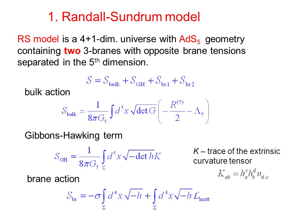
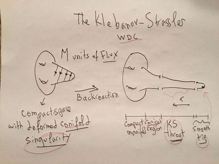
In my last few posts, I showed that the AdS/CFT dual of supergravity on the Klebanov-Strassler warped conifold background is a 4-D N = 1 superconformal gauge theory and the internal compactification-topology and flux-quanta have backgrounds essentially containing KS warped throats: let me relate the KS-throat to Randall-Sundrum geometry
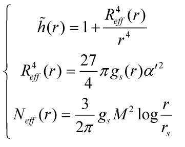
I concluded my last post by inserting the  -metric
into the Klebanov-Tseytlin relation
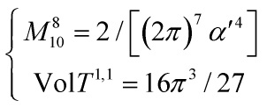
and after differentiating, I derived
which, given the quantization condition
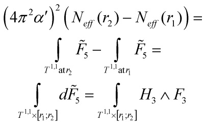
![\[\frac{1}{{4{\pi ^2}\alpha '}}\int_{{S^3}} {{F_3}} = M\]](https://www.georgeshiber.com/wp-content/ql-cache/quicklatex.com-b42fa1d2f4641818e86303063edf1cac_l3.png "Rendered by QuickLaTeX.com")
implies that the scaling  for the non-vanishing components of
  yields
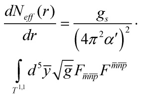
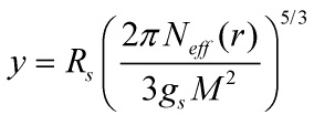
![\[{N_{eff}}(r) = a{g_s}{M^2}\log \left( {r/{r_s}} \right)\]](https://www.georgeshiber.com/wp-content/ql-cache/quicklatex.com-50d165c36a38fbdef967750437d8be1a_l3.png "Rendered by QuickLaTeX.com")
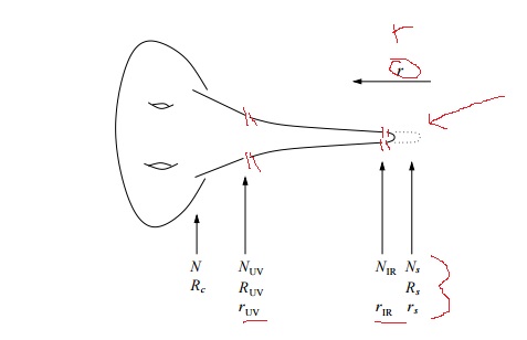
and that will allow us to connect the Klebanov-Strassler throat with the Randall-Sundrum model. Visually, we had …
Now, for a warped conifold throat with geometry  , the curvature radius
  of
of  measures the size of and is constant along the radial direction. The geometry of the KS-warped deformed conifold is also diffeomorphic to and as I demonstrated, there is an effective curvature radius
  which varies slowly with
  .
.
Hence, given the Klebanov-Tseytlin relation above, the correspondence between the Klebanov-Strassler throat and the Randall-Sundrum model can be visualized as …

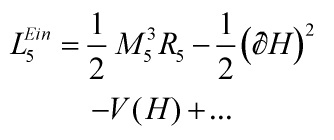
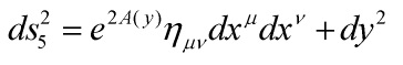
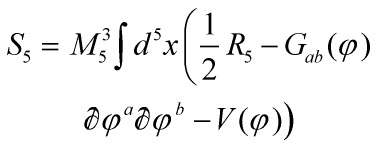
Working in a 5-D Einstein frame with canonically normalized 5-D scalar field  , where the negative 5-D cosmological constant of must be replaced by a vacuum energy density
  , we have
and the backreaction modifies the geometry so as to reproduce our familiar-by-now metric
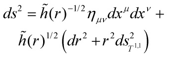
A dimensional reduction of a theory with the metric above to 5-D gives rise to an -dependent coefficient of the 5-D Ricci scalar
![\[M_{5,eff}^3(r)\]](https://www.georgeshiber.com/wp-content/ql-cache/quicklatex.com-2471f3c687e9e3ee5bbce60d5d8d57d4_l3.png "Rendered by QuickLaTeX.com")
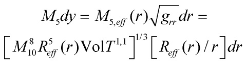
and a model with the above Lagrangian  arises necessarily after a Weyl rescaling by a Tseytlin function of a radially varying scalar field. Now, working with the -dependent infinitesimal distance in units of
  and imposing
with
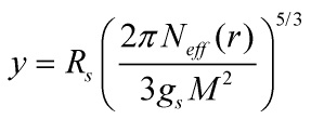
Fixing the constant of integration by choosing  in terms of flux-quanta as
One can write the 5-D metric as
where the warp factor, following from
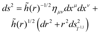
and
and
together with the Weyl rescaling used to get the 5-D Einstein frame, and in light of the Klebanov-Strassler 4-D Lagrangian
reads as
- We are half-way towards deriving our RS-action
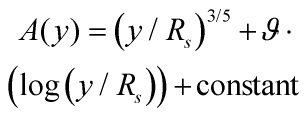
Now, writing the warp factor as
![\[\left\{ {\begin{array}{*{20}{c}}{A(y) = k(y)y}\\{k(y) = R_s^{ - 1}{{\left( {y/{R_s}} \right)}^{ - 2/5}}}\end{array}} \right.\]](https://www.georgeshiber.com/wp-content/ql-cache/quicklatex.com-89bb7315af8f3bdbaba016313d424323_l3.png "Rendered by QuickLaTeX.com")
Let us now use the equation of motion of a scalar field with potential in a warped background
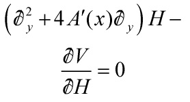
and one can neglect the second-derivative term if the length scale for the variation of is larger than the curvature radius  . We thus get
![\[\frac{{12}}{5}\frac{1}{{{R_s}}}{\left( {\frac{y}{{{R_s}}}} \right)^{ - 1/5}}{\not \partial _y}H = \frac{{\not \partial V}}{{\not \partial H}}\]](https://www.georgeshiber.com/wp-content/ql-cache/quicklatex.com-44455fc9635651b2fcd953ab03a1a622_l3.png "Rendered by QuickLaTeX.com")
From the trace of the Einstein equations for a ‘slowly’ varying scalar field, one obtains a relation between the scalar curvature and the potential energy density
![\[ - \frac{3}{{10}}{R_{icci}} = \frac{{V(H)}}{{M_5^3}}\]](https://www.georgeshiber.com/wp-content/ql-cache/quicklatex.com-25b0eef6b977fdca9e78088892725f38_l3.png "Rendered by QuickLaTeX.com")
and in light of the 5-D metric and warp factor above, becomes
![\[V = \frac{{54}}{{25}}{\left( {\frac{y}{{{R_s}}}} \right)^{ - 4/5}}\frac{{M_5^3}}{{R_s^2}}\]](https://www.georgeshiber.com/wp-content/ql-cache/quicklatex.com-0f504f733a84182ad4bdb113e32c999d_l3.png "Rendered by QuickLaTeX.com")
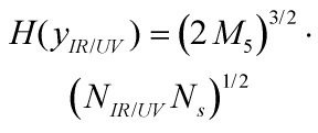
Now using the chain rule
![\[\not \partial V/\not \partial y = \left( {\not \partial V/\not \partial H} \right){\not \partial _y}H\]](https://www.georgeshiber.com/wp-content/ql-cache/quicklatex.com-96e503f76527599707e8eb2cedb5b40a_l3.png "Rendered by QuickLaTeX.com")
we get for
![\[H(y) = {\left( {2{M_5}} \right)^{3/2}}{\left( {\frac{y}{{{R_s}}}} \right)^{3/10}}\]](https://www.georgeshiber.com/wp-content/ql-cache/quicklatex.com-dfe3ff06a30fb8766379afc4cb156dc7_l3.png "Rendered by QuickLaTeX.com")
yielding
![\[\left\{ {\begin{array}{*{20}{c}}{\left| {\not \partial _y^2H} \right| \ll \left| {A'(y){{\not \partial }_y}H} \right|}\\{{{\left( {{{\not \partial }_y}H} \right)}^2} \ll \left| V \right|}\end{array}} \right.\]](https://www.georgeshiber.com/wp-content/ql-cache/quicklatex.com-004cd126f27402c6d558d9f146da59c5_l3.png "Rendered by QuickLaTeX.com")
and the desired functional dependence of  on
on
![\[V(H) = \frac{{864}}{{25}}\frac{{M_5^7}}{{R_5^2}}{H^{ - 8/3}}\]](https://www.georgeshiber.com/wp-content/ql-cache/quicklatex.com-ede3321a394c4657fcd430683714cc0d_l3.png "Rendered by QuickLaTeX.com")
Thus, 5-D gravity coupled to a scalar field H with the potential  reproduces the effective 5-D geometry of the throat
reproduces the effective 5-D geometry of the throatTo get the complete compactification, we need to add tensed IR and UV branes with boundary conditions for to our 5-D model. The explicit relations are
with
![\[{N_s} = \frac{3}{{2\pi }}{g_s}{M^2}\]](https://www.georgeshiber.com/wp-content/ql-cache/quicklatex.com-4d4210e0e4ed41553b0f6a3a19b4a82f_l3.png "Rendered by QuickLaTeX.com")
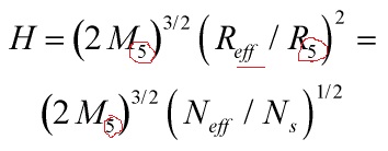
therefore the boundary condition  reproduces the IR end corresponding to a Klebanov-Strassler region with
  units of
  flux,
flux,
and so we have presented a 5-D model, containing gravity with a minimally coupled scalar field, which, upon compactification on an interval with boundary conditions
which provides the 5-D description of the KS throat
visually…
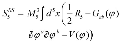
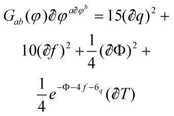
The corresponding nonlinear sigma model can be truncated to a version that involves only four scalars and characterizes the Klebanov-Strassler solution. Letting the fields be denoted by  , then
  measures the volume and
  the ratio of scales between the 2-cycle and the 3-cycle;
  the dilaton, and
  measures the
  potential. Then the 5-D action is
and  collectively denoting the dimensionless scalars , and
…

 and
and  are constants, with proportional to the number of 3-form flux quanta , and with a warped ansatz as in
for the 5-D metric, a solution to the equations of motion is given by the Klebanov-Strassler background
![\[f = \Phi = 0\]](https://www.georgeshiber.com/wp-content/ql-cache/quicklatex.com-5a6c64acfac22fbdab4a1754921a2da8_l3.png "Rendered by QuickLaTeX.com")
and explicitly, at large ,
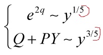
Thus, in terms of the physical quantities we have been using,  and
and  and the leading contribution to the vacuum energy density, whose back-reaction determines the warp factor, is given by the first and last terms of the potential in …
and and the leading contribution to the vacuum energy density, whose back-reaction determines the warp factor, is given by the first and last terms of the potential in …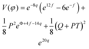
…evaluated on the solution
U-Kähler modulus analysis is next.
