The Lindblad Master Equation, Feynman-Kac Formula, and the Measurement Problem

By George Shiber Sunday, March 12, 2017Friday, October 26, 2018 In Cosmology, Mathematical Physics, Mathematics, Philosophy Of Physics, Philosophy Of Science, Physics, Time Feynman-Kac Formula, Quantum Cohomology

Any adequate account of how micro-causality and quantum coherence can explain the emergent-property of spacetime and how the Wheeler-DeWitt problem of time can be solved must incorporate a theory of how the Lindblad master equation solves the Markov quantum fluctuation problem as well as demonstrate how the quantum Jarzynski-Hatano-Sasa relation can be homologically defined globally for both, Minkowski space and Friedmann-Robertson-Walker generalized Cartan space-times. This is a step towards those goals. Consider a wave-function $\left| {{\psi _t}^{S,m,c}} \right\rangle$ and the entropic quantum entanglement relation of the total system consisting of ‘S’, ‘m’ and the quantum-time measuring clock ‘c’ subject to Heisenberg’s UP. It follows then that the probability that any given initial state $\left| {\psi _t^{S,m,c}} \right\rangle$ evolves for a time $T$ that undergoes $N$ jumps during intervals $\delta t$ centered at times ${t_1},...,{t_N}$ is given by:

$\begin{array}{l}{\left( {2\delta t{\kappa ^2}/G} \right)^N}{\rm{Tr}}\left\{ {{e^{ - i{{\tilde H}_{eff}}\left( {T - {t_N}} \right)}}} \right. \cdot \\\hat a{e^{ - i{{\hat H}_{eff}}}}\left( {{t_N} - {t_{N - 1}}} \right)\hat a...\,\hat a{e^{ - i{{\hat H}_{eff}}t}}\\ \times \left| {\psi _t^{S,m,c}} \right\rangle \left\langle {\psi _t^{S,m,c}} \right|{e^{i{{\tilde H}^\dagger }_{eff}{t_1}}}{{\hat a}^\dagger }...\,\left. {{{\hat a}^\dagger }{e^{i{{\tilde H}^\dagger }_{eff}\left( {T - {t_N}} \right)}}} \right\}\end{array}$

So, the master equation:

$\begin{array}{l}{{\dot \rho }_{00}} = - i\left[ {{{\hat H}_0},{\rho _{00}}} \right] + \frac{{2{\kappa ^2}}}{G}\hat a{\rho _{00}}{{\hat a}^\dagger }\\ - \frac{{{\kappa ^2}}}{G}{{\hat a}^\dagger }\hat a{\rho _{00}} - \frac{{{\kappa ^2}}}{G}{\rho _{00}}{{\hat a}^\dagger }\hat a\end{array}$

is valid iff the Markovian approximation is faithful and valid only on time-scales longer than $1/{\Gamma _1}$ , hence the jump occurs during an interval $\delta t \sim 1/{\Gamma _1}$ centered on ${t_i}$ . Therefore, with the Hamiltonian:

${\hat H_I} = \kappa \left( {{{\hat a}^\dagger } \otimes \hat b + \hat a \otimes {{\hat b}^\dagger }} \right)$

where $\left( {\hat a,\hat b} \right);\left( {{{\hat a}^\dagger },{{\hat b}^\dagger }} \right)$ are the lowering/raising operators for the system and output mode respectively, it follows that the total system satisfies the master equation:

$\begin{array}{c}\dot \rho = - i\left[ {\hat H,\rho } \right] + {\Gamma _1}\hat b\rho {{\hat b}^\dagger } - \frac{{{\Gamma _1}}}{2}{{\hat b}^\dagger }\hat b\rho \\ - \frac{{{\Gamma _1}}}{2}\rho {{\hat b}^\dagger }\hat b + {\Gamma _2}{\sigma _z}\rho {\sigma _z} - {\Gamma _2}\rho \\ \equiv L_s^L\rho \end{array}$

where the Pauli operator ${\sigma _z}$ acts on the output mode and $L_s^L$ is the Liouville superoperator. Given that it is a linear equation, it has a solution given as:

$\rho ({t_2}) = \exp \left\{ {L_s^L\left( {{t_2} - {t_1}} \right)} \right\}\rho ({t_1})$

and so the evolution of the density matrix ${\rho _t}$ is given by the Lindblad master equation:

$\begin{array}{l}{\partial _t}{\rho _t} = - i\left[ {{H_t},{\rho _t}} \right] + \sum\limits_{i = 1}^I {\left( {{V_i}{\rho _t}V_i^\dagger } \right.} \\\left. { - \frac{1}{2}V_i^\dagger {V_i}{\rho _t} - \frac{1}{2}{\rho _t}V_i^\dagger {V_i}} \right)\end{array}$

where

$- \left[ {{H_t},X} \right]$

is the conservative part and ${{H_t}}$ is the time-dependent Hamiltonian of the system and the other terms refer to the bath of the interactive system and reflect the effect of measurements, and ${V_i}$ are the Kraus-operators, not necessarily hermitians and are typically explicitly dependent on time. The Kraus number $I$ depends on the bath. In the case where the system is a closed one, the Kraus operators vanish identically and the Lindblad master equation reduces to the quantum version of the Liouville equation, giving us:

${\partial _t}{\rho _t} = L_t^\dagger {\rho _t}$

with $L_t^\dagger$ the Lindbladian superoperator acting on the density matrix and determines its dynamics. The associated space of operators is equipped with a Hilbert-Schmidt scalar product:

$\left( {Y,X} \right) = {\rm{Tr}}\left( {{Y^\dagger }X} \right)$

with ${{Y^\dagger }}$ the hermitian conjugate of $Y$ . We now define a pair of adjoint superoperators ${L^\dagger }$ and $L_t^\dagger$ as follows:

$\begin{array}{l}\left( {Y,L,X} \right) = {\rm{Tr}}\left( {{Y^\dagger }\left( {L,X} \right)} \right) = \\\left( {L_t^\dagger Y,X} \right) = {\rm{Tr}}\left( {{{\left( {L_t^\dagger Y} \right)}^\dagger }X} \right)\end{array}$

Hence, we have:

$\begin{array}{l}{L_t}X = i\left[ {{H_t},X} \right] + \sum\limits_{i = 1}^I {\left( {V_i^\dagger } \right.} X{V_i} - \\\frac{1}{2}V_i^\dagger {V_i}X - \left. {\frac{1}{2}XV_i^\dagger {V_i}} \right)\end{array}$

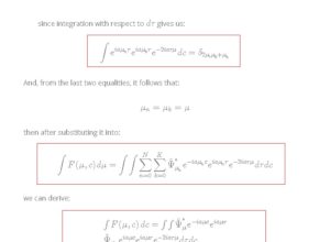
with the trace-conservation property:

$\left\{ {\begin{array}{*{20}{c}}{{L_t}1 = 0}\\{{L_t}\left( {{X^\dagger }} \right) = {{\left( {{L_t}X} \right)}^\dagger }}\end{array}} \right.$

The solve quantum Master equation:

${\partial _t}{\rho _t} = L_t^\dagger {\rho _t}$

one typically introduces an evolution superoperator $P_0^t$ defined implicitly by:

${\rho _t} = {\left( {P_0^t} \right)^\dagger }{\pi _0}$

where ${\pi _0}$ is the initial-time-density-matrix, and the superoperator evolution is given by:

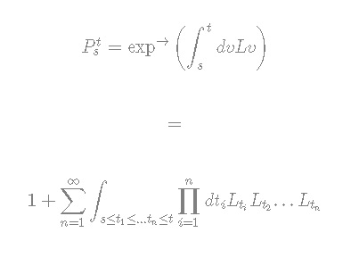
$P_s^t = {\exp ^ \to }\left( {\int_s^t {dvLv} } \right)$

$=$

$1 + \sum\limits_{n = 1}^\infty {\int_{s \le {t_1} \le ...{t_n} \le t} {\prod\limits_{i = 1}^n {d{t_i}} } } {L_{{t_i}}}{L_{{t_2}}}...{L_{{t_n}}}$

And in this time-ordered exponential, time is monotonically increasing from left to right.

To prove:

${\rho _t} = {\left( {P_0^t} \right)^\dagger }{\pi _0}$

note that it is true at $t = 0$ since $P_0^0$ is the identity operator. Thus, from:

$P_s^t = {\exp ^ \to }\left( {\int_s^t {dvLv} } \right)$

$=$

$1 + \sum\limits_{n = 1}^\infty {\int_{s \le {t_1} \le ...{t_n} \le t} {\prod\limits_{i = 1}^n {d{t_i}} } } {L_{{t_i}}}{L_{{t_2}}}...{L_{{t_n}}}$

one finds that:

$\frac{d}{{dt}}P_s^t = P_s^t{L_t}$

holds, and leads to:

$\frac{d}{{dt}}{\rho _t} = \left( {L_t^\dagger {{\left( {P_0^t} \right)}^\dagger }} \right){\pi _0} = L_t^\dagger {\rho _t}$

entailing that it satisfies the Lindblad equation:

${\partial _t}{\rho _t} = L_t^\dagger {\rho _t}$

with initial condition ${\pi _0}$ . Now, for the evolution operator, one writes an expression for multi-time correlations for distinct observables. For:

$0 \le {t_1} \le {t_2} \le ... \le {t_N} \le t$

the time-ordered correlation is:

${\left\langle {{O_1}\left( {{t_1}} \right){O_2}\left( {{t_2}} \right)...{O_N}\left( {{t_N}} \right)} \right\rangle _{{\pi _0}}}$

$=$

${\rm{Tr}}\left( {{\pi _0}P_0^{{t_1}}{O_1}P_{{t_1}}^{{t_2}}{O_2}...P_{{t_{N - 1}}}^{{t_N}}{O_N}} \right)$

and can be evaluated in the Heisenberg representation formalism by using the full Hamiltonian of the system plus its environment. Since the total density matrix factorizes at each observation time and the weak Lindblad Master equation coupling assumption holds in that formalism, the time-ordered two-time correlation function satisfies an evolution equation which is the dual to:

${\partial _t}{\rho _t} = L_t^\dagger {\rho _t}$

our proof is complete.

Now note that in:

${\left\langle {{O_1}\left( {{t_1}} \right){O_2}\left( {{t_2}} \right)...{O_N}\left( {{t_N}} \right)} \right\rangle _{{\pi _0}}}$

$=$

${\rm{Tr}}\left( {{\pi _0}P_0^{{t_1}}{O_1}P_{{t_1}}^{{t_2}}{O_2}...P_{{t_{N - 1}}}^{{t_N}}{O_N}} \right)$

the operator ${\pi _0}$ represents the initial density matrix of the system and the superoperator $P_{{t_i}}^{{t_{i + 1}}}$ acts on all terms to its right.

Thus, we have the crucial equation:

$\left\{ {\begin{array}{*{20}{c}}{L_0^\dagger {\pi _0} = 0}\\{L_t^\dagger {\pi _t} = 0}\end{array}} \right.$

which for systems prepared in a thermal state at:

$T = \frac{1}{{k\beta }}$

with $k$ the Boltzmann-constant, we have:

${\pi _0} = Z_0^{ - 1}\exp \left( { - \beta H\left( 0 \right)} \right)$

For closed systems, one has:

${\pi _t} = Z_t^{ - 1}\exp \left( { - \beta {H_t}} \right)$

which holds for any Markovian process weakly coupled with a thermal bath at $T = {\beta ^{ - 1}}$ provided the bath satisfies the KMS condition. Here, we shall consider generally, far from equilibrium cases, where ${\pi _t}$ is not given by the canonical Gibbs-Boltzmann formula.

Deriving the Jarzynski-Hatano-Sasa identity for quantum Markovian dynamics

Even though the density-matrix ${\pi _t}$ does not obey the Lindblad equation, it is a solution of the deformation-evolution equation:

${\partial _t}{\pi _t} = {\left( {{L_t} + \pi _t^{ - 1}\left( {{\partial _t}{\pi _t}} \right)} \right)^\dagger }{\pi _t}$

Now, let us define non-stationarity via the operator:

${W_t} = - {\left( {{\pi _t}} \right)^{ - 1}}\left( {{\partial _t}{\pi _t}} \right)$

Define the modified superoperator as such:

${L_{t,1}} = {L_t} + {\left( {{\pi _t}} \right)^{ - 1}}\left( {{\partial _t}{\pi _t}} \right) = {L_t} - {W_t}$

where ${W_t}$ acts by multiplication on the left. Such a superoperator corresponds to the auxiliary dynamics:

${\partial _t}{\rho _t} = L_{t,1}^\dagger {\rho _t}$

and yields a modified evolution superoperator via:

$P_{s,1}^t = {\exp ^ \to }\left( {\int_s^t {{L_{v,1}}} dv} \right)$

$=$

${\exp ^ \to }\left( {\int_s^t {\left( {{L_v} + \pi _v^{ - 1}\left( {{\partial _v}{\pi _v}} \right)} \right)dv} } \right)$

Given:

${\partial _t}{\pi _t} = {\left( {{L_t} + \pi _t^{ - 1}\left( {{\partial _t}{\pi _t}} \right)} \right)^\dagger }{\pi _t}$

we can derive:

${\partial _t}{\pi _t} = L_{t,1}^\dagger {\pi _t}$

with solution:

${\pi _t} = {\left( {P_{0,t}^t} \right)^\dagger }{\pi _t}$

Now, for any observable $A$ , such a solution gives us:

${\rm{Tr}}\left( {{\pi _0}P_{t,1}^1A} \right) = {\rm{Tr}}\left( {{\pi _t}A} \right)$

One can derive a quantum variant of the Jarzynski-Hatano-Sasa relation by connecting the auxiliary evolution superoperator $P_{0,1}^t$ to the initial evolution superoperator $P_s^t$ . In order to do that, we need to prove an extension of the Feynman-Kac formula: write the Dyson-Schwinger expansion of $P_{0,1}^t$ , with ${W_t}$ a perturbation of the Lindbladian ${L_t}$ :

$P_{0,1}^t = {\sum\limits_n {\left( { - 1} \right)} ^n}\int_{0 \le {t_1} \le {t_2} \le ... \le {t_n} \le t} {\prod\limits_{i = 1}^n {d{t_i}} } P_0^{{t_1}}{W_{{t_n}}}P_{{t_1}}^{{t_2}}{W_{{t_2}}}...P_{{t_{N - 1}}}^{{t_N}}{W_{_{{t_N}}}}P_{{t_N}}^t$

where $P_{{t_i}}^{{t_i} + 1}$ acts on all the terms to its right. Now, insert the Dyson-Schwinger expansion into the r.h.s. of:

${\rm{Tr}}\left( {{\pi _0}P_{t,1}^1A} \right) = {\rm{Tr}}\left( {{\pi _t}A} \right)$

and we get:

${\rm{Tr}}\left( {{\pi _0}P_{0,1}^tA} \right) = \sum\limits_n {{{\left( { - 1} \right)}^n}} \int_{0 \le {t_1} \le {t_2} \le ... \le {t_n} \le t} {\prod\limits_{i = 1}^n {d{t_i}} }$

$\times$

${\rm{Tr}}\left( {{\pi _0}P_{0,1}^t{W_{{t_1}}}P_{{t_1}}^{{t_2}}{W_{{t_2}}}...P_{{t_{N - 1}}}^{{t_N}}W{t_N}P_{{t_N}}^tA} \right)$

Reformulate the trace within the scope of the integrals as a multi-time correlation via:

${\left\langle {{O_1}\left( {{t_1}} \right){O_2}\left( {{t_2}} \right)...{O_N}\left( {{t_N}} \right)} \right\rangle _{{\pi _0}}}$

$=$

${\rm{Tr}}\left( {{\pi _0}P_0^{{t_1}}{O_1}P_{{t_1}}^{{t_2}}{O_2}...P_{{t_{N - 1}}}^{{t_N}}{O_N}} \right)$

and we get:

${\rm{Tr}}\left( {{\pi _0}P_{0,1}^tA} \right) = \sum\limits_n {{{\left( { - 1} \right)}^n}} \int_{0 \le {t_1} \le {t_2} \le ... \le {t_n} \le t} {\prod\limits_{i = 1}^n {d{t_i}} }$

$\circ$

${\left\langle {{W_{{t_1}}}\left( {{t_1}} \right){W_{{t_2}}}\left( {{t_2}} \right)...{W_{{t_N}}}\left( {{t_N}} \right)A\left( t \right)} \right\rangle _{{\pi _0}}}$

and by linearity and the relation ${O_i} = {W_{{t_i}}}$ , we get a reduction to:

${\rm{Tr}}\left( {{\pi _0}P_{0,1}^tA} \right)$

$=$

${\left\langle {\left\{ {\sum\limits_n {{{\left( { - 1} \right)}^n}\int_{0 \le {t_1} \le {t_2} \le ... \le {t_n} \le t} {\prod\limits_{i = 1}^n {d{t_i}} } {W_{{t_1}}}\left( {{t_1}} \right){W_{{t_2}}}\left( {{t_2}} \right)...{W_{{t_N}}}\left( {{t_N}} \right)} } \right\}A} \right\rangle _{{\pi _0}}}$

where the terms inside the brackets are summable as a time-ordered exponential:

${\rm{Tr}}\left( {{\pi _0}P_{0,1}^tA} \right)$

$=$

${\left\langle {{{\exp }^ \to }\left( { - \int_0^t {{W_v}\left( v \right)dv} } \right)A\left( t \right)} \right\rangle _{{\pi _0}}}$

This is an extension of the Feynman-Kac formula for quantum Markov semi-groups.

and by non-commutativity of the operator algebra, the Feynman-Kac exponential is replaced by a time-ordered exponential. Hence, one gets:

${\rm{Tr}}\left( {{\pi _t}A} \right)$

$=$

${\left\langle {{{\exp }^ \to }\left( { - \int_0^t {{W_v}\left( v \right)dv} } \right)A\left( t \right)} \right\rangle _{{\pi _0}}}$

and is a quantum extension of the classical Jarzynski-Hatano-Sasa identity

If we set $A = \hat 1'$ , the above identity reduces to:

${\left\langle {{{\exp }^ \to }\left( { - \int_0^t {{W_v}\left( v \right)dv} } \right)} \right\rangle _{{\pi _0}}} = 1$

given that ${\rm{Tr}}\left( {{\pi _t}} \right) = 1$ holds, and is a quantum measurement number-raising and book-keeping formula for correlation functions.

Now, from a first order expansion of:

${\left\langle {{{\exp }^ \to }\left( { - \int_0^t {{W_v}\left( v \right)dv} } \right)} \right\rangle _{{\pi _0}}} = 1$

we can deduce a generalized fluctuation-dissipation theorem valid in the Heisenberg-vicinity of a quantum non-equilibrium steady state.

The case of a closed isolated system determined by a time-dependent Hamiltonian, the Lindbladian reduces to the Liouville operator:

${L_t}X = i\left[ {{H_t},X} \right]$

with unitary evolution. For a closed system, the evolution superoperator acts on observables as follows:

$P_0^tX = {\left( {U_0^t} \right)^\dagger }X\,U_0^t$

with:

$U_0^t \equiv {\exp ^ \leftarrow }\int_0^t {dv} \left( { - i{H_v}} \right)$

The image of X under the superoperator operator defines the Heisenberg operator ${X^\mathcal{H}}\left( t \right)$ with $\mathcal{H}$ representing the Heisenberg operator:

$P_0^tX = {X^\mathcal{H}}\left( t \right)$

Since the superoperator is multiplicative, the r.h.s. of:

${\left\langle {{O_1}\left( {{t_1}} \right){O_2}\left( {{t_2}} \right)...{O_N}\left( {{t_N}} \right)} \right\rangle _{{\pi _0}}}$

$=$

${\rm{Tr}}\left( {{\pi _0}P_0^{{t_1}}{O_1}P_{{t_1}}^{{t_2}}{O_2}...P_{{t_{N - 1}}}^{{t_N}}{O_N}} \right)$

for multi-time correlations can be evaluated and one gets:

${\left\langle {{O_1}\left( {{t_1}} \right){O_2}\left( {{t_2}} \right)...{O_N}\left( {{t_N}} \right)} \right\rangle _{{\pi _0}}}$

$=$

${\rm{Tr}}\left( {{\pi _0}O_1^\mathcal{H}\left( {{t_1}} \right)O_2^\mathcal{H}\left( {{t_2}} \right)...O_N^\mathcal{H}\left( {{t_N}} \right)} \right)$

Hence, for a closed system the quantum Jarzynski-Hatano-Sasa relation is:

${\rm{Tr}}\left( {{\pi _t}A} \right)$

$=$

${\rm{Tr}}\left( {{\pi _0}{{\exp }^ \to }\left( { - \int_0^t {{W_v}{{\left( v \right)}^\mathcal{H}}dv} } \right){A^\mathcal{H}}\left( t \right)} \right)$

From multiplicativity and:

$P_0^tX = {X^\mathcal{H}}\left( t \right)$

we have:

${\exp ^ \to }\left( { - \int_0^1 {{W_v}{{\left( v \right)}^\mathcal{H}}dv} } \right) = {\left( {{\pi _0}} \right)^{ - 1}}\pi _t^\mathcal{H}\left( t \right)$

and given that we have ${\pi _t} = Z_t^{ - 1}\exp \left( { - \beta {H_t}} \right)$ , we can derive:

${W_v}{\left( v \right)^\mathcal{H}} = - {\left( {\pi _v^{ - 1}} \right)^\mathcal{H}}\left( v \right){\left( {{\partial _v}{\pi _v}} \right)^\mathcal{H}}\left( v \right)$

Now, from $A = \hat 1'$ , we get the Kurchan-Tasaki quantum Jarzynski relation for closed systems. Moreover, since we have the commutation relation:

$\left[ {{H_v},{\partial _v}{H_v}} \right] = 0$

we can derive:

$\frac{{{Z_t}}}{{{Z_0}}}{\rm{Tr}}\left( {{\pi _t}A} \right)$

$=$

${\rm{Tr}}\left( {{\pi _0}{{\exp }^ \to }\left( { - \beta \int_0^t {{{\left( {{\partial _v}{H_v}} \right)}^\mathcal{H}}\left( v \right)dv} } \right){A^\mathcal{H}}\left( t \right)} \right)$

and for the critical case where $A = 1$ holds, the Hänggi-Talkner quantum-Jarzynski relation for closed systems reduces to:

${\rm{Tr}}\left( {{\pi _0}{{\exp }^ \to }\left( { - \beta \int_0^t {{{\left( {{\partial _v}{H_v}} \right)}^\mathcal{H}}\left( v \right)dv} } \right)} \right) = \frac{{{Z_t}}}{{{Z_0}}}$

For open systems, which are of more foundational interest, it follows from:

${\rm{Tr}}\left( {{\pi _t}A} \right)$

$=$

${\left\langle {{{\exp }^ \to }\left( { - \int_0^t {{W_v}\left( v \right)dv} } \right)A\left( t \right)} \right\rangle _{{\pi _0}}}$

that the generalized fluctuation-dissipation theorem is valid in the vicinity of any quantum non-equilibrium steady state. To see that, take a perturbation of the Lindbladian ${L_0}$ of the form:

${L_t} = {L_0} - {h^a}\left( t \right){M_a}$

with

${h^a}\left( t \right)$

time-dependent perturbations. The density matrix ${\pi _t}$ satisfying:

$L_{t, \cdot }^\dagger {\pi _t} = 0$

is given by:

${\pi _t} = {\pi _0} + {h^a}\left( t \right){\varepsilon _a}$

with ${\varepsilon _a}$ satisfying:

$L_{0, \cdot }^\dagger {\varepsilon _a} = M_{a, \cdot }^\dagger {\pi _0}$

and the non-stationary operator becomes:

$\left\{ {\begin{array}{*{20}{c}}{{W_t} = - {{\dot h}^a}\left( t \right){D_a}}\\{{D_a} \equiv \pi _0^{ - 1}{\varepsilon _a}}\end{array}} \right.$

By differentiating, we get:

${\left. {\frac{{\delta \left\langle {A\left( t \right)} \right\rangle }}{{\delta {h^a}\left( v \right)}}} \right|_{h = 0}} = \frac{d}{{dv}}{\left\langle {{D_a}\left( v \right)A\left( t \right)} \right\rangle _{{\pi _0}}}$

where:

$\frac{d}{{dv}}{\left\langle {{D_a}\left( v \right)A\left( t \right)} \right\rangle _{{\pi _0}}}$

is taken with respect to the unperturbed density matrix ${\pi _0}$ .

Lindbladian time-reversal dynamics

Time reversal on the states $\psi$ of the Hilbert space in quantum mechanics is implemented by an anti-linear anti-unitary operator ${\mathord{\buildrel{\lower3pt\hbox{$\scriptscriptstyle\smile$}} \over U} ^\neg }$ satisfying:

$\left\{ {\begin{array}{*{20}{c}}{{{\mathord{\buildrel{\lower3pt\hbox{$\scriptscriptstyle\smile$}} \over U} }^\neg }^2 = 1}\\{{{\mathord{\buildrel{\lower3pt\hbox{$\scriptscriptstyle\smile$}} \over U} }^\neg } = {{\mathord{\buildrel{\lower3pt\hbox{$\scriptscriptstyle\smile$}} \over U} }^\neg }^{ - 1} = {{\mathord{\buildrel{\lower3pt\hbox{$\scriptscriptstyle\smile$}} \over U} }^\neg }^\dagger }\end{array}} \right.$

for spin-0 particles without a magnetic field, ${\mathord{\buildrel{\lower3pt\hbox{$\scriptscriptstyle\smile$}} \over U} ^\neg }$ is the complex conjugation operator: that is, by time reversal, the Schrödinger wave-function $\psi$ becomes ${\psi ^ * }$ . In the scenario where there is a magnetic field, time-inversion must be augmented by requiring that the reversed system evolves with vector potential ${A^R} = - 1$ . Time reversal of Hilbert space observables is hence implemented by a superoperator $K$ that acts on an operator $X$ as such:

$KX = {\mathord{\buildrel{\lower3pt\hbox{$\scriptscriptstyle\smile$}} \over U} ^\neg }X{\mathord{\buildrel{\lower3pt\hbox{$\scriptscriptstyle\smile$}} \over U} ^\neg }^{ - 1}$

Hence, as promised, $K$ is multiplicative, anti-unitary, and satisfies:

$\left\{ {\begin{array}{*{20}{c}}{{K^2} = 1}\\{K = {K^{ - 1}} = {K^\dagger }}\end{array}} \right.$

We are finally in a position to define time-reversal for a quantum Markov process. Take a constant Lindbladian $L$ lying in a steady state with density-matrix $\pi$ . Note that the superoperator ${L^R}$ that determines the reversed process is given by:

${L^R} = K{\pi ^{ - 1}}{L^\dagger }\pi K$

and the micro-reversibility condition is:

$\left\{ {\begin{array}{*{20}{c}}{{L^R} = L}\\ \equiv \\{K{\pi ^{ - 1}}{L^\dagger }\pi K = L}\end{array}} \right.$

yielding the finite-time formula:

$\pi P_0^T = K{\left( {P_0^T} \right)^\dagger }K\pi$

which, given two arbitrary observables $A$ , $B$ , is equivalent to:

${\rm{Tr}}\left( {{B^\dagger }\pi P_0^TA} \right) = {\rm{Tr}}\left( {\left( {K{A^\dagger }} \right)\pi P_0^T\left( {KB} \right)} \right)$

Hence, we can see that the stationary density matrix associated with the time-reversed dynamics is given by:

${\pi ^R} = K\pi$

given that:

${\left( {{L^R}} \right)^\dagger }\left( {K\pi } \right) = 0$

We have therefore the following crucial Lindbladian:

$L_{{t^ * }}^R = K\pi _t^{ - 1}L_t^\dagger {\pi _t}K\;\,;\,\,\,{t^ * } = T - 1$

From this Lindbladian equation and ${L_t}1 = 0$ , we obtain:

${\left( {L_{{t^ * }}^R} \right)^\dagger }K{\pi _t} = 0$

and:

$\pi _{{t^ * }}^R = K{\pi _t}$

thus connecting the Lindbladian distribution of the time-reversed system with that of the classical system.

Now, applying:

to the time-reversed system, we find that the evolution superoperator of the time-reversed system is given by:

$P_s^{t,R} = {\exp ^ \to }\left( {\int_s^t {dv} L_v^R} \right)$

with multi-time correlations:

${\left\langle {{O_1}\left( {{t_1}} \right){O_2}\left( {{t_2}} \right)...{O_N}\left( {{t_N}} \right)} \right\rangle ^R}$

$=$

${\rm{Tr}}\left( {\pi _0^RP_0^{{t_1},R}{O_1}P_{{t_1}}^{{t_2},R}{O_2}...P_N^{{t_N},R}{O_N}} \right)$

Continuing with our proof, let $\alpha$ be a scalar such that $0 \le \alpha \le 1$ and define two $\alpha$ -deformed superoperators, that act on an observable X as follows:

$\left\{ {\begin{array}{*{20}{c}}{{L_t}\left( \alpha \right)}\\{L_t^R}\end{array}} \right.{ \triangleright _{acting\,\,on}}:X$

Def.:

${L_t}\left( \alpha \right)X\left( {{L_t} + \alpha \pi _t^{ - 1}{\partial _t}{\pi _t}} \right)X$

and:

$L_t^R\left( \alpha \right)X\left( {L_t^R + \alpha {{\left( {\pi _t^R} \right)}^{ - 1}}{\partial _t}\pi _t^R} \right)X$

Now, the superoperators ${L_t}\left( \alpha \right)$ interpolate between ${L_t}$ and ${L_{t,1}}$ when $\alpha$ varies from $0$ to $1$ . Likewise, $L_t^R\left( \alpha \right)$ is an interpolation from $L_t^R$ to $L_{t,1}^R$ . The corresponding $\alpha$ -deformed evolution superoperators are given by:

$P_s^t\left( \alpha \right) = {\exp ^ \to }\left( {\int_s^t {dv\,{L_v}\left( \alpha \right)} } \right)$

and:

$P_s^{t,R}\left( \alpha \right) = {\exp ^ \to }\left( {\int_s^t {dv\,L_v^R\left( \alpha \right)} } \right)$

Crucially, they satisfy the following duality relation that lies at the heart of the quantum fluctuation theorem:

${\pi _0}P_0^T\left( \alpha \right) = {\left[ {{\pi _T}KP_0^{T,R}\left( {1 - \alpha } \right)K} \right]^\dagger }$

hence, we can derive the following for the unitary operator:

${\left. {{{\mathord{\buildrel{\lower3pt\hbox{$\scriptscriptstyle\smile$}} \over U} }^\neg }_t = {\pi _0}P_0^t\left( \alpha \right)\pi _t^{ - 1} = 1} \right|_{t = 0}} = 1$

and satisfies:

$\begin{array}{l}{\partial _t}{{\mathord{\buildrel{\lower3pt\hbox{$\scriptscriptstyle\smile$}} \over U} }^\neg }_t = {\pi _0}P_0^t\pi _t^{ - 1}\left( {{\pi _1}{L_t}\left( \alpha \right)\pi _1^{ - 1}{\partial _t}{\pi _1}\pi _t^{ - 1}} \right)\\ = {{\mathord{\buildrel{\lower3pt\hbox{$\scriptscriptstyle\smile$}} \over U} }^\neg }_t\left( {{\pi _1}{L_t}\pi _1^{ - 1} + \left( {\alpha - 1} \right){\partial _t}{\pi _1}\pi _t^{ - 1}} \right)\\ = {{\mathord{\buildrel{\lower3pt\hbox{$\scriptscriptstyle\smile$}} \over U} }^\neg }_t{\left( {KL_{{t^ * }}^R\left( {1 - \alpha } \right)K} \right)^\dagger }\end{array}$

So we can write the operator as:

${{\mathord{\buildrel{\lower3pt\hbox{$\scriptscriptstyle\smile$}} \over U} }^\neg }_t = {\exp ^ \to }{\left( {\int_0^T {dvL_v^R\left( {1 - \alpha } \right)K} } \right)^\dagger }$

$=$

${\left( {K{{\exp }^ \to }\int_0^T {dvL_v^R\left( {1 - \alpha } \right)K} } \right)^\dagger } = {\left( {KP_0^{T,R}\left( {1 - \alpha } \right)K} \right)^\dagger }$

Using the duality above to any pair of observables $A$ and $B$ , and the multiplicative property and anti-unitary of $K$ , our proof is finalized by the following relation:

${\rm{Tr}}\left( {{B^\dagger }{\pi _0}P_0^T\left( \alpha \right)A} \right) = {\rm{Tr}}\left( {\left( {K{A^\dagger }} \right)\pi _0^RP_0^{T,R}\left( {1 - \alpha } \right)\left( {KB} \right)} \right)$

This is precisely the equation that axiomatically captures the essence of the quantum fluctuation theorem that explains quantum decoherence and undergirds the solution to the measurement problem, up to a Yukawa-Higgs S-matrix coupling constant. To see this, express it in terms of quantum density-matrix stochasticity via the expectation-operator:

$\left\langle {{{\left( {{\pi _0}B\pi _0^{ - 1}} \right)}^\dagger }\left( 0 \right){{\exp }^ \to }\left( { - \alpha \int_0^T {dv{W_v}\left( v \right)} } \right)} \right\rangle$

$=$

${\left\langle {{{\left( {\pi _0^R\left( {KA} \right){{\left( {\pi _0^R} \right)}^{ - 1}}} \right)}^\dagger }\left( 0 \right){{\exp }^ \to }\left( { - \left( {1 - \alpha } \right)\int_0^T {dvW_v^R\left( v \right)} } \right)\left( {KB} \right)\left( T \right)} \right\rangle ^R}$

with $W_t^R$ the asymmetric reversed operator given by:

$W_t^R = - {\left( {\pi _t^R} \right)^{ - 1}}{\partial _t}\pi _t^R$

and is closed with Hamiltonian

$H_{{t^ * }}^R = K{H_t}$

and the evolution operator satisfies:

${\mathord{\buildrel{\lower3pt\hbox{$\scriptscriptstyle\smile$}} \over U} ^{\neg ,}}_0^{T,R} = {K_\parallel }{\left( {{{\mathord{\buildrel{\lower3pt\hbox{$\scriptscriptstyle\smile$}} \over U} }^{\neg ,}}_0^T} \right)^\dagger }$

by the Boltzmann law, the above equation in the Heisenberg representation is:

${\rm{Tr}}\left( {{B^\dagger }{\pi _0}\exp \left( {\beta H_0^\mathcal{H}\left( 0 \right)} \right)} \right)\exp \left( {\left( { - \beta H_0^\mathcal{H}\left( T \right)} \right){A^\mathcal{H}}\left( T \right)} \right)$

$=$

$\frac{{{Z_T}}}{{{Z_0}}}{\rm{Tr}}{\left( {K\left( {{A^\dagger }} \right)\pi _0^R\left( {{{\mathord{\buildrel{\lower3pt\hbox{$\scriptscriptstyle\smile$}} \over U} }^{\neg ,}}_0^{T,R}} \right)} \right)^\dagger }K\left( B \right){{\mathord{\buildrel{\lower3pt\hbox{$\scriptscriptstyle\smile$}} \over U} }^{\neg ,}}_0^{T,R}$