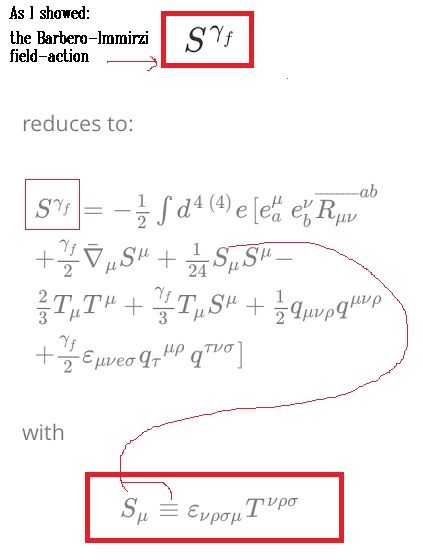
The Nieh–Yan Action and Barbero-Immirzi Hamiltonian Analysis

By George Shiber Tuesday, November 1, 2016Friday, October 26, 2018 In Cosmology, Loop Quantum Gravity, Mathematical Physics, Mathematics, Philosophy Of Physics, Physics Barbero-Immirzi Hamiltonian Analysis, Barbero–Immirzi field

I will derive the following: the Nieh–Yan action, in the context of Barbero-Immirzi Hamiltonian analysis, allows the phase-space of General Relativity to be determined by Ashtekar-Barbero variables, and as to why this is deep and crucial for the viability of LQG is a topic for another post. Recall how I showed that the Barbero–Immirzi field action:

$\begin{array}{l}{S^{{\gamma _f}}} = - \frac{1}{2}\int {{d^4}{\,^{(4)}}} e\left[ {e_a^\mu } \right.e_b^\nu {\overline {{R_{\mu \nu }}} ^{ab}}\\ + \frac{{{\gamma _f}}}{2}{{\bar \nabla }_\mu }{S^\mu } + \frac{1}{{24}}{S_\mu }{S^\mu } - \\\frac{2}{3}{T_\mu }{T^\mu } + \frac{{{\gamma _f}}}{3}{T_\mu }{S^\mu } + \frac{1}{2}{q_{\mu \nu \rho }}{q^{\mu \nu \rho }}\\ + \frac{{{\gamma _f}}}{2}{\varepsilon _{\mu \nu e\sigma }}{q_\tau }^{\mu \rho }\left. {{q^{\tau \nu \sigma }}} \right]\end{array}$

with

${S_\mu } \equiv {\varepsilon _{\nu \rho \sigma \mu }}{T^{\nu \rho \sigma }}$

and

${\bar \nabla _\mu }$

the torsion-less metric-compatible covariant derivative, induces contortion spin-connections by solving:

${\gamma _f}$

and hence:

${S^{{\gamma _f}}}$

generalizes to:

$\begin{array}{l}S_{NY}^{{\gamma _f}} = - \frac{1}{2}\int {{d^4}} x{\,^{(4)}}e\,e_a^\mu e_b^\nu {R_{\mu \nu }}^{ab} - \\\frac{1}{4}\int {{d^4}} x{\,^{(4)}}e{\gamma _f}\left( {{\eta _{ab}}} \right.T_{\mu \nu }^aT_{\rho \sigma }^a - \\e_a^\mu e_b^\nu \varepsilon _{cd}^{ab}\left. {{R_{\mu \nu }}^{cd}} \right)\end{array}$

Thus, the second integral is the Nieh-Yan topological invariant and connects to the Holst term, yielding:

$\begin{array}{l}^\dagger S_{NY}^{{\gamma _f}} = - \frac{1}{2}\int {{d^4}} x{\,^{(4)}}e\left[ {e_a^\mu } \right.e_b^\nu {\overline {{R_{\mu \nu }}} ^{ab}}\\ + \frac{{{\gamma _f}}}{2}{{\bar \nabla }_\mu }{S^\mu } + \frac{1}{{24}}{S_\mu }{S^\mu } - \frac{1}{3}{T_\mu }{T^\mu }\\ + \frac{1}{2}{q_{\mu \nu \rho }}\left. {{q^{_{\mu \nu \rho }}}} \right]\end{array}$

After varying the action with respect to the irreducible components of:

$\left\{ {\begin{array}{*{20}{c}}{{S^\mu }}\\{{T^\nu }}\\{{q^{\rho \sigma \tau }}}\end{array}} \right.$

we obtain:

$\left\{ {\begin{array}{*{20}{c}}{{\partial _\mu }{\gamma _f} - \frac{1}{6} - {S_\mu } = 0}\\{{T_\mu } = 0}\\{{q_{\mu \nu \rho }} = 0}\end{array}} \right.$

Inserting into:

$^\dagger S_{NY}^{{\gamma _f}}$

one gets the effective action:

$\begin{array}{l}S_{eff}^{{\gamma _f}} = - \frac{1}{2}\int {{d^4}} x{\,^{(4)}}ee_a^\mu e_b^\nu {\overline {{R_{\mu \iota }}} ^{ab}} + \\\frac{3}{4}\int {{d^4}} x{\,^{(4)}}e{\partial _\alpha }{\gamma _f}{\partial ^\alpha }{\gamma _f}\end{array}$

giving us an equivalence with the Hilbert-Palatini torsion-free action and thus solving the gauge-free accessibility problem as well as the 4-D uplifting problem caused by invariance under rescaling symmetry and translational symmetry.

Now, since the phase-space has symplectic structure:

$\left\{ {K_\alpha ^i\left( {t,x} \right),E_j^\gamma \left( {t,x'} \right)} \right\} = \delta _\alpha ^\gamma \delta _j^i\delta \left( {x,x'} \right)$

and

$\left\{ {{\gamma _f}\left( {t,x} \right),\prod \left( {t,x'} \right)} \right\} = \delta \left( {x,x'} \right)$

It thus follows that the total BI-field Hamiltonian:

${H_{tot}} = \int {{d^3}} x\left( {{ \wedge ^i}} \right.{\tilde R_i} + {N^\alpha }\widetilde {{H_\alpha }} + \left. {N\widetilde H} \right)$

with

$\left\{ {\begin{array}{*{20}{c}}{{ \wedge ^i}}\\{{N^\alpha }}\\N\end{array}} \right.$

the Lagrange multipliers, obeys:

${\partial _{{o_t}}}{\gamma _f}^\phi \left\{ {{H_{tot}},{\gamma _f}^\phi } \right\}$

where

$\left\{ {\;,\;} \right\}$

is the Poisson bracket satisfying:

$\begin{array}{l}\left\{ {E_i^a\left( x \right),A_b^i\left( x \right)} \right\} = \delta _b^a\delta _j^i\left( {x,y} \right) = \\\left\{ {\pi _i^\alpha \left( x \right),\omega _b^{(3)i}\left( y \right)} \right\}\end{array}$

with

${\partial _{{0_t}}}{\gamma _f}^\phi$

being the time-evolution of the BI-field and

$\phi$

an arbitrary field.

Now, the Einstein field equations with the Immirzi parameter and a cosmological constant are given by the BF-type action (EIBF):

$\begin{array}{l}S\left[ {B,\omega ,\phi ,\mu } \right] = \int_M {\left[ {\left( {{B^{IJ}} + \frac{1}{\gamma } * {B^{IJ}}} \right)} \right.} \\ \wedge {F_{IJ}}[\omega ] - {\phi _{IJKL}}{B^{IJ}} \wedge {B^{KL}} - \mu {\phi _{IJKL}}{\varepsilon ^{IJKL}}\\ + \mu \lambda + {l_1}{B_{IJ}} \wedge \left. {{B^{IJ}} + {l_2}{B_{IJ}} \wedge * {B^{IJ}}} \right]\end{array}$

where

${B^{IJ}}$

is a set of 6 2-forms

$\left( {{B^{IJ}} = - {B^{IJ}}} \right)$

and ${F_{IJ}}$ being the curvature for the connection ${\omega _{IJ}}$ with components:

${F_{\mu \nu IJ}} = 2\left( {{\partial _{\left[ {_\mu {\omega _\nu }} \right]IJ}} + {\omega _{\left[ {\mu {{\left| I \right.}^K}{\omega _\nu }} \right]KJ}}} \right)$

with cosmological constant terms:

$\left\{ {\begin{array}{*{20}{c}}\lambda \\{{l_1}}\\{{l_2}}\end{array}} \right.$

and ${\phi _{IJKL}}$ the internal tensor constraining the B-field with symmetries:

${\phi _{IJKL}} = {\phi _{KLIJ}} = - {\phi _{JIKL}} = - {\phi _{IJLK}}$

$\mu$ a 4-form and $\gamma$ is the Immirzi parameter. As is standard, $*$ is the internal Hodge dual:

$\begin{array}{l} * {U_{IJ}} = (1/2){\varepsilon _{IJKL}}{U^{KL}}\\{\rm{with:}}\quad \quad {{\rm{U}}_{IJ}} = - {U_{IJ}}\end{array}$

with:

${\varepsilon _{0123}} = 1$

Now, since one can integrate the Immirzi parameter into the theory, the following identity can be derived:

$^{\left( \gamma \right)}{U_{IJ}} \equiv {U_{IJ}} + \frac{1}{\gamma } * {U_{IJ}}$

with inverse transformation:

${U_{IJ}} = \frac{{{\gamma ^2}}}{{{\gamma ^2} - \sigma }}\left( {^{\left( \gamma \right)}{U_{IJ}} - \frac{1}{\gamma }{ * ^{\left( \gamma \right)}}{U_{IJ}}} \right)$

Combining with the EIBF-action:

one can derive the following identities:

$^{\left( \gamma \right)}{U_{IJ}}{V^{IJ}} = {U_{IJ}}^{\left( \gamma \right)}{V^{IJ}}$

$\left( {{U_{\left[ {\left. I \right|} \right.}}^K{V_{K\left| {\left. J \right]} \right.}}} \right){ = ^{\left( \gamma \right)}}{U_{\left[ {\left. I \right|} \right.}}{V_{K\left| {\left. J \right]} \right.}} = {U_{\left[ {\left. I \right|} \right.}}{K^K}{V_{K\left| {\left. J \right]} \right.}}$

$\begin{array}{l} * \left( {{U_{\left[ {\left. I \right|} \right.}}^K{V_{K\left| {\left. J \right]} \right.}}} \right) = * {U_{\left[ {\left. I \right|} \right.}}^K{V_{K\left| {\left. J \right]} \right.}}\\ = {U_{\left[ {\left. I \right|} \right.}}^K * {V_{K\left| {\left. J \right]} \right.}}\end{array}$

– The first step in the Hamiltonian analysis of the EIBF-action is that, given that the total BI-field Hamiltonian:

${H_{tot}} = \int {{d^3}} x\left( {{ \wedge ^i}} \right.{\tilde R_i} + {N^\alpha }\widetilde {{H_\alpha }} + \left. {N\widetilde H} \right)$

obeys:

${\partial _{{o_t}}}{\gamma _f}^\phi \left\{ {{H_{tot}},{\gamma _f}^\phi } \right\}$

where

$\left\{ {\;,\;} \right\}$

is the Poisson bracket, the Hamiltonian takes the following form:

$\begin{array}{l}S\left[ {{\omega _a}{,^{\left( \gamma \right)}}{\Pi ^a},\tilde N,{N^a},\xi ,{\varphi _{ab}},{\psi _{ab}}} \right]\\ = \int_\mathbb{R} {dt} \int_\Omega {{d^3}} x\left( {^{\left( \gamma \right)}{\Pi ^{aIJ}}} \right.{{\dot \omega }_{aIJ}} + \tilde N\tilde H\\ + {N^a}{{\tilde H}_a} + {\xi _{IJ}}{\wp ^{IJ}} + {\varphi _{ab}}{\Phi ^{ab}} + \left. {{\psi _{ab}}{\Psi ^{ab}}} \right)\end{array}$

with:

$^{\left( \gamma \right)}{\Pi ^{aIJ}}$

the canonically conjugate momenta with respect to the connection:

${\omega _{abIJ}}$

and the following holds:

${\Pi ^{aIJ}}{ = _{def}}\frac{1}{2}{\tilde \eta ^{abc}}{B_{bc}}^{IJ}$

and

${\tilde \eta ^{abc}}$

is an antisymmetric tensor density of weight +1. Now, the Lagrange multipliers:

$\left\{ {\begin{array}{*{20}{c}}{{ \wedge ^i}}\\{{N^\alpha }}\\N\end{array}} \right.$

allow us to deduce the following crucial EIBF constraints:

${\wp ^{IJ}}: = {D_a}^{\left( \gamma \right)}{\Pi ^{aIJ}} \approx 0$

${\tilde H_a}: = \frac{1}{2}{\Pi ^{bIJ}}{\,^{\left( \gamma \right)}}{F_{baIJ}} \approx 0$

$\begin{array}{c}\tilde H: = \frac{1}{4}{{\tilde \eta }^{abc}}{h_{ad}} * {\Pi ^{dIJ}}{\,^{\left( \gamma \right)}}{F_{bcIJ}}\\ + 2\Lambda h \approx 0\end{array}$

${\Phi ^{ab}}: = - \sigma * {\Pi ^{aIJ}}{\Pi ^b}_{IJ} \approx 0$

and

${\Psi ^{ab}}: = 2{h_{cf}}{\tilde \eta ^{\left( {a\left| {cd} \right.} \right.}}{\Pi ^f}_{IJ}{D_d}{\Pi ^{\left| {\left. b \right)IJ} \right.}} \approx 0$

and

$\Lambda = 3{l_2} - \sigma \lambda /4$

the cosmological constant, and ${D_a}$ is the SO(1,3) covariant derivative:

$\left( {{D_a}{\Pi ^{bIJ}} = {\partial _a}{\Pi ^{bIJ}} + \omega _a^I{\,_K}{\Pi ^{bIJ}} - \omega _a^I{\,_K}{\Pi ^{bKI}}} \right)$

and $h$ is the determinant of the spatial metric ${h_{ab}}$ whose inverse ${h^{ab}}$ satisfies:

$h{h^{ab}} = \frac{\sigma }{2}{\Pi ^{aIJ}}{\Pi ^b}_{IJ}$

Now, one can use the Dirac-method to eliminate some canonical variables from the theory thus reducing the solution to the equations:

${\Phi ^{ab}}: = - \sigma * {\Pi ^{aIJ}}{\Pi ^b}_{IJ} \approx 0$

${\Psi ^{ab}}: = 2{h_{cf}}{\tilde \eta ^{\left( {a\left| {cd} \right.} \right.}}{\Pi ^f}_{IJ}{D_d}{\Pi ^{\left| {\left. b \right)IJ} \right.}} \approx 0$

to the original Holstsian phase-space. Noting that the following:

${\Pi ^{a0i}} = {E^{ai}}$

is a solution, it follows that ${E^{ai}}$ is invertible with inverse ${E_{ai}}$ , and the following relation:

$h{h^{ab}} = \frac{\sigma }{2}{\Pi ^{aIJ}}{\Pi ^b}_{IJ}$

reduces to:

$h{h^{ab}} = {\eta _{ij}}{E^{ai}}{E^{bj}}$

with:

${\eta _{ij}}: = \left( {1 + \sigma {\chi _k}{\chi ^k}} \right){\delta _{ij}} - \sigma {\chi _i}{\chi _i}$

Similarly, one can use

${\Phi ^{ab}}: = - \sigma * {\Pi ^{aIJ}}{\Pi ^b}_{IJ} \approx 0$

${\Psi ^{ab}}: = 2{h_{cf}}{\tilde \eta ^{\left( {a\left| {cd} \right.} \right.}}{\Pi ^f}_{IJ}{D_d}{\Pi ^{\left| {\left. b \right)IJ} \right.}} \approx 0$

in order to collapse the symplectic structure to:

$\begin{array}{l}\int_\Omega {{d^3}} x\left( {^{\left( \gamma \right)}{\Pi ^{aIJ}}{{\dot \omega }_{aIJ}}} \right) = \\\int_\Omega {{d^3}} x\left( {{\Pi ^{aIJ}}{{\frac{\partial }{{\partial t}}}^{\left( \gamma \right)}}{\omega _{aIJ}}} \right) = \\2\int_\Omega {{d^3}} x\left( {{E^{ai}}{{\dot A}_{ai}} + {\zeta _i}{{\dot \chi }^i}} \right)\end{array}$

such that the following hold:

${A_{ai}}:{ = ^{\,\left( \gamma \right)}}{\omega _{a0i}}{ + ^{\,\left( \gamma \right)}}{\omega _{aIJ}}{\chi ^j}$

${\zeta _i}:{ = ^{\left( \gamma \right)}}{\omega _{aij}}{E^{aj}}$

hence, the phase space variables:

$\left\{ {\begin{array}{*{20}{c}}{\left( {{A_{ai}},{E^{ai}}} \right)}\\{\left( {{\chi ^i},{\zeta _i}} \right)}\end{array}} \right.$

obey the Poisson brackets:

$\left\{ {{A_{ai}}(x),{E^{bj}}(y)} \right\} = \frac{1}{2}\delta _a^b\delta _i^j{\delta ^3}\left( {x,y} \right)$

$\left\{ {{\chi ^j}(x),{\zeta _j}(y)} \right\} = \frac{1}{2}\delta _j^i{\delta ^3}\left( {x,y} \right)$

Now, since:

${\zeta _i}:{ = ^{\left( \gamma \right)}}{\omega _{aij}}{E^{aj}}$

is an inhomogeneous linear system of equations for the unknowns $^{\left( \gamma \right)}{\omega _{aij}}$ , with general solution:

$^{\left( \gamma \right)}{\omega _{aij}} = \frac{1}{2}{\varepsilon _{ijk}}{E_{al}}{M^{kl}} - {E_{a\left[ {_i{\zeta _j}} \right]}}$

From:

${A_{ai}}:{ = ^{\,\left( \gamma \right)}}{\omega _{a0i}}{ + ^{\,\left( \gamma \right)}}{\omega _{aIJ}}{\chi ^j}$

we can derive:

$^{\left( \gamma \right)}{\omega _{a0i}} = {A_{ai}}{ - ^{\left( \gamma \right)}}{\omega _{aij}}{\chi ^j}$

thus, we have a linear map:

$\left( {{A_{ai}},{\zeta _i},{M^{ij}}} \right) \to \left( {^{\left( \gamma \right)}{\omega _{a0i}}{,^{\left( \gamma \right)}}{\omega _{aij}}} \right)$

whose inverse map is:

$\left( {^{\left( \gamma \right)}{\omega _{a0i}}{,^{\left( \gamma \right)}}{\omega _{aij}}} \right) \to \left( {{A_{ai}},{\zeta _i},{M^{ij}}} \right)$

together with:

${M^{ij}} = {E^{a{{\left( {^i{\varepsilon ^j}} \right)}^{kl}}}}^{\left( \gamma \right)}{\omega _{akl}}$

Consistency conditions with the Holst action impose on us:

$\begin{array}{l}{M^{ij}} = \frac{1}{{1 + \sigma {\chi _m}{\chi ^m}}}\left[ {\left( {{f^k}_k + \sigma {f_{kl}}{\chi ^k}{\chi ^l}} \right)} \right.{\delta ^{ij}}\\ + \left( {\sigma {f^k}_k - \sigma {f_{kl}}{\chi ^k}{\chi ^l}} \right){\chi ^i}{\chi ^j} - \\{f^{ij}} - {f^{ji}} - \sigma \left( {{f^{ik}}{\chi ^j} + {f^{jk}}{\chi ^i} + {f^{kj}}{\chi ^i}} \right)\left. {{\chi _k}} \right]\end{array}$

by substituting, we can derive:

${\Psi ^{ab}} = {T^{abij}}{f_{ij}} + {G^{ab}} \approx 0$

with:

$\begin{array}{l}{f_{ij}} = - {\varepsilon _{ikl}}{E^{ak}}\left[ {\left( {1 - \sigma {\gamma ^{ - 2}}} \right)} \right.{E_{bj}}{\partial _a}{E^{bl}}\\\left. { + \sigma {\chi ^l}{A_{aj}}} \right] + \frac{\sigma }{\gamma }\left( {{E^{ak}}{A_{ak}}{\delta _{ij}} - {A_{ai}}{E^a}_j + {\zeta _i}{\chi _j}} \right)\end{array}$

Now, we are in a position to rewrite the remaining constraints in:

as phase-space variables, thus the Gauss constraint splits into boost and rotational parts as follows:

$\begin{array}{l}\wp _{boost}^i: = {\wp ^{0i}} = {\partial _a}\left( {{E^{ai}} + \frac{\sigma }{\gamma }{\varepsilon ^i}_{jk}{E^{ai}}{\chi ^k}} \right)\\ + \,2\sigma {A_{aj}}{E^{a\left[ {^j{\chi ^i}} \right]}} + \sigma {\zeta _j}{\chi ^j}{\chi ^i} + {\zeta ^i}\end{array}$

and

$\begin{array}{l}\wp _{rot}^i: = \frac{1}{2}{\varepsilon ^i}_{jk}{\wp ^{jk}} = {\partial _a}\left( {{\varepsilon ^i}_{jk}{E^{aj}}{\chi ^k} + \frac{1}{\gamma }{E^{aj}}} \right)\\ - {\varepsilon ^i}_{jk}\left( {A_a^j{E^{ak}} - {\zeta ^j}{\chi ^k}} \right)\end{array}$

yielding the vector and scalar constraints:

$\begin{array}{l}{{\tilde H}_a} = 2{E^{bi}}{\partial _{\left[ {_b{A_a}} \right]i}} - {\zeta _i}{\partial _a}{\chi ^i} + \\\frac{{{\gamma ^2}}}{{{\gamma ^2} - \sigma }}\left[ {2\sigma } \right.{E^{b\left[ {^i{\chi ^j}} \right]}}{A_{ai}}{A_{bj}} - \\ - {A_{ai}}\left( {{\zeta ^i} + \sigma {\zeta _j}{\chi ^j}{\chi ^i}} \right) + \\\frac{\sigma }{\gamma }{\varepsilon _{ijk}}\left( {{E^{bi}}A_b^j + {\zeta ^i}{\chi ^j}} \right)\left. {A_a^k} \right]\end{array}$

and

$\begin{array}{l}\tilde H = - \sigma {E^{ai}}{\chi _i}{{\tilde H}_a} + \left( {1 + \sigma {\chi _k}{\chi ^k}} \right)\\ \cdot \left( {{E^{ai}}{\partial _a}{\zeta _i} + \frac{1}{2}{\zeta _i}{E^{ai}}{E^{bj}}{\partial _a}{E_{bj}}} \right)\\ - \frac{{\sigma {\gamma ^2}}}{{{\gamma ^2} - \sigma }}\left\{ {\left( {1 + \sigma {\chi _l}{\chi ^l}} \right)} \right.\left[ {{E^{ai}}} \right.{E^{bj}}{A_{a\left[ {\left. i \right)} \right.}}{A_{b\left[ {\left. j \right)} \right.}}\\ + {\zeta _i}{\chi ^i}{A_{aj}}{E^{aj}} + \frac{3}{4}{\left( {{\zeta _i}{\chi ^i}} \right)^2} + \frac{3}{4}\sigma {\zeta _i}{\zeta ^i}\\ - \frac{1}{\gamma }{\varepsilon _{ijk}}{E^{ai}}A_a^j\left. {{\zeta ^k}} \right] - \frac{\sigma }{4}{\left( {f_i^i} \right)^2} + \\\frac{\sigma }{2}{f^{ij}}{f_{\left( {ij} \right)}} - \frac{1}{2}{f_{ij}}{\chi ^i}{\chi ^j}\left( {f_k^k - \frac{\sigma }{2}{f_{kl}}{\chi ^k}{\chi ^l}} \right)\\ + \frac{1}{4}\left( {{f_{ij}} + {f_{ji}}} \right)\left( {{f^{ik}} + {f^{ki}}} \right)\left. {{\chi ^j}\chi k} \right\}\\ + 2\Lambda \left( {1 + \sigma {\chi _k}{\chi ^k}} \right)E\end{array}$

where:

$E: = \det \left( {{E^{ai}}} \right)$

relates to $h$ via:

${h^2} = {\left( {1 + \sigma {\chi _k}{\chi ^k}} \right)^2}{E^2}$

Hence, our phase space is now determined by 12, down from 24, canonical pairs:

$\left\{ {\left( {{A_{ai}},{E^{ai}}} \right),\left( {{\chi ^i},{\zeta _i}} \right)} \right\}$

and to construct the Barbero’s formulation one must demand that the variables ${E^{ai}}$ constitute a densitized triad for the spatial metric ${h_{ab}}$ , that is:

${\chi ^i} = 0$

Up until now, our formalism and theory is fully diffeomorphism and Lorentz invariant, however, one must break the Lorentz group $SO\left( {1,3} \right)$ down to its compact subgroup $SO\left( 3 \right)$ in order to derive the Ashtekar-Barbero variables, and this is accomplished by choosing the time-gauge:

${\chi ^i} = 0$

The solution of the second-class constraints is thus given by:

$\left\{ {\begin{array}{*{20}{c}}{{\Pi ^{a0i}} = {E^{ai}}}\\{{\Pi ^{aij}} = 0}\end{array}} \right.$

and:

$^{\left( \gamma \right)}{\omega _{a0i}} = {A_{ai}}$

$^{\left( \gamma \right)}{\omega _{aij}} = {\varepsilon _{ijk}}\left[ {\left( {1 - \sigma {\gamma ^2}} \right)\Gamma _a^k + \sigma {\gamma ^{ - 1}}A_a^k} \right]$

where ${\Gamma _{ai}}$ is the rotational part of ${\omega _{aIJ}}$ , that is:

${\Gamma _{ai}}: = \frac{1}{2}{\varepsilon _{ijk}}{\omega _a}^{jk}$

which allow us to derive:

$\wp _{boost}^i = {\partial _a}{E^{ai}} + {\varepsilon ^{ijk}}\left[ {\left( {1 - \sigma {\gamma ^{ - 2}}} \right){\Gamma _{ak}} + \sigma {\gamma ^{ - 1}}{A_{ak}}} \right]{E^a}_j$

$\wp _{rot}^i = {\gamma ^{ - 1}}{\partial _a}{E^{ai}} - {\varepsilon ^{ijk}}{A_{aj}}{E^a}_k$

${\Psi ^{ab}} = - 4\sigma {\varepsilon _{ijk}}{E^{ci}}{E^{\left( {\left. a \right|k} \right.}}\left( \begin{array}{l}{\partial _c}{E^{\left| {\left. b \right)j} \right.}}\\ - {\varepsilon ^{ilm}}{\Gamma _{cl}}{E^{\left| {\left. b \right)} \right.}}_m\end{array} \right)$

Combining them, one gets:

$\begin{array}{l}\frac{{{\gamma ^2}}}{{{\gamma ^2} - \sigma }}\left( {\wp _{boost}^i - \frac{\sigma }{\gamma }\wp _{rot}^i} \right) = \\{\partial _a}{E^{ai}} + {\varepsilon ^{ijk}}{\Gamma _{ak}}{E^a}_j = 0\end{array}$

and together with:

$\wp _{rot}^i = {\gamma ^{ - 1}}{\partial _a}{E^{ai}} - {\varepsilon ^{ijk}}{A_{aj}}{E^a}_k$

we get the following solution:

${\Gamma _{ai}} = {\varepsilon _{ijk}}\left( {{\partial _{\left[ {_b{E_a}} \right]}}^j + {E_a}^{\left[ {\left. l \right|} \right.}{E^{c\left[ {\left. j \right|} \right.}}{\partial _b}{E_{cl}}} \right){E^{bk}}$

And here’s the crucial point: this is the spin-connection of the densitized triad ${E^{ai}}$

and satisfies the following 3 relations:

${\wp ^i} = {\gamma ^{ - 1}}{\ddot \not D_a}{E^{ai}}$

${\tilde H_a} = {E^{bi}}{F_{bai}} + \left( {1 - \sigma {\gamma ^{ - 2}}} \right)\left( \begin{array}{l}\gamma {A_{ai}}\\ - {\Gamma _{ai}}\end{array} \right){\wp ^i}$

$\begin{array}{l}\tilde H = \frac{\sigma }{{2\gamma }}{\varepsilon _{ijk}}{E^{aj}}{E^{bk}}\left[ {{F_{ab}}^i} \right. + \left( {\sigma \gamma - } \right.\\\left. {{\gamma ^{ - 1}}} \right)\left. {{R_{ab}}^i} \right] + 2\Lambda E\end{array}$

with:

$\ddot \not D{E^{ai}}: = {\partial _a}{E^{ai}} - \gamma {\varepsilon ^{ijk}}{A_{aj}}{E^a}_k$

and:

$\left\{ {\begin{array}{*{20}{c}}{{F_{abi}}}\\{{R_{abi}}}\end{array}} \right.$

are the curvatures of the connections:

$\left\{ {\begin{array}{*{20}{c}}{{A_{ai}}}\\{{\Gamma _{ai}}}\end{array}} \right.$

obeying the following equations:

${F_{abi}} = 2{\partial _{\left[ {_a{A_b}} \right]\,i}} - \gamma {\varepsilon _{ijk}}{A_a}^j{A_b}^k$

${R_{abi}} = 2{\partial _{\left[ {_a{\Gamma _b}} \right]\,i}} - {\varepsilon _{ijk}}{\Gamma _a}^j{\Gamma _b}^k$

$\left\{ {\begin{array}{*{20}{c}}{\sigma = - 1}\\{\gamma = \pm i}\end{array}} \right.$

Hence, the reformulation of the phase space of General Relativity in terms of our canonical variables recovers the Ashtekar formulation given

our Hamiltonian:

${H_{tot}} = \int {{d^3}} x\left( {{ \wedge ^i}} \right.{\tilde R_i} + {N^\alpha }\widetilde {{H_\alpha }} + \left. {N\widetilde H} \right)$

The Nieh–Yan Action and Barbero-Immirzi Hamiltonian Analysis

${\gamma _f}$

${S^{{\gamma _f}}}$

$^\dagger S_{NY}^{{\gamma _f}}$

${\partial _{{0_t}}}{\gamma _f}^\phi$

$^{\left( \gamma \right)}{\Pi ^{aIJ}}$

${\omega _{abIJ}}$

${\tilde \eta ^{abc}}$

And here’s the crucial point: this is the spin-connection of the densitized triad ${E^{ai}}$

Hence, the reformulation of the phase space of General Relativity in terms of our canonical variables recovers the Ashtekar formulation given

and given the Nieh–Yan action: we can describe the phase space of general relativity in terms of the Ashtekar-Barbero variables

The Barbero-Immirzi Field and the Nieh–Yan Topological Invariant

Quantum Non-Locality and Wave Function Collapse

About Me

Social Networks

Archives

Login Below

Photo Gallery

And here’s the crucial point: this is the spin-connection of the densitized triad

Hence, the reformulation of the phase space of General Relativity in terms of our canonical variables recovers the Ashtekar formulation given

and given the Nieh–Yan action: we can describe the phase space of general relativity in terms of the Ashtekar-Barbero variables

The Barbero-Immirzi Field and the Nieh–Yan Topological Invariant

Quantum Non-Locality and Wave Function Collapse

RELATED

F-theory as the Modular Equivariant 12-D Lift of Type-IIB String Theory

Exceptional Field Theory and M-Theory on Kovalev TCS G2-Manifolds

The Wess–Zumino–Witten–Novikov Model, Taub-NUT Spaces, and M-Theory

About Me

Social Networks

Archives

Login Below

Photo Gallery

And here’s the crucial point: this is the spin-connection of the densitized triad ${E^{ai}}$