A Källén–Lehmann D-3-Brane Clifford Harmonic Derivation Of The Particle-Spectrum

By George Shiber Thursday, August 6, 2015Sunday, June 23, 2019 In Grand Unification Physics, M Theory, Mathematical Physics, Physics, Super String Theory, Supersymmetry AdS/CFT Duality, bosons

This … is… magic: “The number 24 appearing in Ramanujan’s function is also the origin of the miraculous cancellations occurring in String Theory … each of the 24 modes in the Ramanujan function corresponds to a physical vibration of a string. Whenever the string executes its complex motions in space-time by splitting and recombining, a large number of highly complex mathematical identities must be satisfied. These are precisely the mathematical identities discovered by Ramanujan … the string vibrates in ten dimensions because it requires generalized Ramanujan functions in order to remain self-consitent. ~ Michio Kaku, in Hyperspace : A Scientific Odyssey Through Parallel Universes, Time Warps, and the Tenth Dimension (1995) Ch.7 Superstrings!

I will show you something truly remarkable in M-theory in a second, magical really – like you need more magic after reading the Kaku quote above about Ramanujan and string theory. But first, recall that I showed how one can derive the initial singularity ‘creation’ relation in a finite way describing a holographic elimination of space-time, and hence, by GR, gravity, via squaring:

$\frac{d}{{dt}}\left( {\underbrace {\int_0^{\delta {f_K}} {\frac{{\frac{d}{{d{t^ \circ }}}{\Psi ^{wf}}_{U\left| {_{INST}} \right.}(eh)}}{{\alpha ({t^ \circ })}}} }_{Creation}\,\, + \underbrace {\int_{{\delta _f}}^{{f_K}} {\frac{{\frac{d}{{d{t^ \circ }}}{\Psi ^{wf}}_{U\left| {_{INST}} \right.}{{(eh)}^{2\pi i\xi t}}}}{{\alpha ({t^ \circ })}}} }_{QuantumGravity}} \right)d\,\Omega {({\phi _{si}})^2}dt$

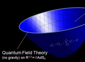
One can then deduce that space-time and gravity are holographic entropic projections of the Fukaya category of the Sasaki-Einstein AdS/CFT space. This was possible because the LHS of the Hodge equation:

${\int_{\widetilde M} {\left\langle {{d^E}\Psi _{U\left| {_{INST}} \right.}^{wf}(eh){,^F}\Psi _{U\left| {_{INST}} \right.}^{wf}(eh} \right\rangle } _{k + 1}}d\,\Omega {({\phi _{si}})^{k + 1}} = {\int_{\partial M} {\left\langle {\Psi _{U\left| {_{INST}} \right.}^{wf}(eh),\delta {\,^F}{\Psi _{U\left| {_{ti}} \right.}}} \right\rangle } _k}d\,\Omega {({\phi _{si}})^k}$

admits a 10-dimensional metric, derived in a second, with ${\Psi _{U\left| {_{ti}} \right.}} \equiv {\Psi ^{wf}}_{U\left| {_{ti}} \right.}$ the wavefunction of the universe at t = i, and $^F{\Psi ^{wf}}_{U\left| {_{ti}} \right.}$ its Fourier transform and $\Psi _{U\left| {_{INST}} \right.}^{wf}(eh)$ the Einstein-Hilbert actional wavefuntion of the universe coupled with the instanton, which is a field configuration that is concentrated at a point in time in the worldvolume of the Dirichlet brane of the corresponding string variable, defined on the Hilbert space corresponding to $Ad{S_5} \times E_S^5$ . The critical 10-dimensional metric takes the form:

$m_{INST}^{10} \equiv ds_{10}^2 = {\Omega ^2}{\phi _{INST}}ds_{1,4}^2 + ds_5^2$

where $\Omega$ is a conformal warping factorial determined by the $E_S^5$ Calabi-Yau conic tip angles, and $ds_5^2$ is the Fukaya metric that symmetrically deforms on the corresponding transverse space. Note, $m_{INST}^{10}$ is $SO(4) \times SO(2)$ invariant, and hence one can topologically split the Dirichlet data:

$\gamma = \delta d{s^2} = \frac{{d{z^2}}}{{{z^2}}}\not \partial {\phi _{si}} + \frac{1}{{{z^2}}}{\varphi _{ij}}(z,x)d{x^i}d{x^j}d\,\Omega {({\phi _{si}})^2}$

with:

${\varphi _{ij}}(z,x) = {z^{(d - \Delta )\exp ( - {\phi _{si}})}}{\phi _{si}}(z,x)$

into the metric $d\,\Omega \left( {{\phi _{INST}}} \right)_3^2$ on a ${S^3}$ and 2 other angles $\theta$ and $\varphi$ that cohomologically stabilize $E_S^5$ . The solution is then:

$\left\{ {\begin{array}{*{20}{c}}{\Omega \left( {{\phi _{INST}}^2} \right) = \frac{{{{\overline X }_1}^{1/2}}}{\rho }}\\{{{\overline X }_1} = {{\cos }^2}\theta + {\rho ^6}{{\sin }^2}\theta }\end{array}} \right.$

with

$ds_5^2 = \Omega {\left( {{\phi _{INST}}} \right)^2}\frac{{{l^2}}}{{{\rho ^2}}}\left[ {d{\theta ^2} + \frac{{{{\sin }^2}\theta }}{{{{\overline X }_1}}}d{\varphi ^2} + \frac{{{\rho ^6}{{\cos }^2}\theta }}{{{{\overline X }_1}}}d\,\Omega _3^2} \right]$

The key is that the supergravity Sasaki-Einstein fields all vanish, with the exception of:

$\left\{ {\begin{array}{*{20}{c}}{{e^\Phi } = {g_s}}\\{{C_{\left( 4 \right)}}\frac{{{e^{4A}}{{\overline X }_1}}}{{{g_s}{\rho ^2}}}dt \wedge d{x^1} \wedge d{x^2} \wedge d{x^3}}\end{array}} \right.$

So far, we have really ‘beautiful’ geometry, but there is a lot of physics to be gotten that describes the Coulomb branch of the moduli space of $N = 4\quad {\rm{SuSy}}$ with gauge-invariance. Basically, it is interpolating N branes apart, away from the origin $u = 0$ . Since the Sasaki-Einstein branes are all BPS, no brane can dynamically transverse any other, and only 16 super-charges are present, which entails that the moduli space is flat. In the $Ad{S_5} \times E_S^5$ frame, there will be some D-3 branes whose world-volume action:

$\begin{array}{c}S_V^{D3} = - \tau {\int_{\partial E_S^5} {{d^4}\xi {\rm{det}}} ^{1/2}}\left[ {{G_{ab}}\,d\,\Omega {{\left( {{\phi _{INST}}} \right)}^3} + {e^{ - \Phi /2}}{F_{ab}}} \right]\\ + \,{\mu _3}\int_{\partial E_S^5} {\left( {{C_{\left( 4 \right)}} + {C_{\left( 2 \right)}} \wedge F + \frac{1}{2}{C_{\left( 0 \right)}}F \wedge F} \right)} \end{array}$

with:

${F_{ab}} = {B_{ab}} + 2\pi \,{\alpha ^\dagger }{F_{ab}}$

and $\partial E_S^5$ is Sasaki-Einstein boundary, with D-3 brane coordinates $\left\{ {{\xi ^0},...,{\xi ^3}} \right\}$ , with ${\mu _3}$ and ${\tau _3}$ the R-R charge and tension of the D-3 brane:

${\mu _3} = {\tau _3}{g_3} = {\left( {2\pi } \right)^{ - 3}}{\left( {{\alpha ^\dagger }} \right)^{ - 2}}$

exhibits NS-NS Einstein ‘brane vanishing’, and thus the metric dimensionally reduces on the moduli space, and is given by:

$\begin{array}{c}ds_{\partial E_S^5}^2 = \frac{{{\tau _3}}}{2}\frac{{{{\overline X }_1}{e^{2A}}}}{{{\rho ^2}}}\left[ {d{\tau ^2}} \right. + \frac{{{l^2}}}{{{\rho ^2}}}\left( {d{\theta ^2} + \frac{{{{\sin }^2}\theta }}{{{{\overline X }_1}}}d{\varphi ^2}d\,\Omega {{\left( {{\phi _{INST}}} \right)}^2}} \right)\\ + \,\,\frac{{{\rho ^6}{{\cos }^2}\theta }}{{{{\overline X }_1}}}d\left. {\Omega _3^2} \right]\end{array}$

and is certainly not flat: this constitutes a serious cosmological problem for any quantum gravity theory. The solution lies in a dual gauge-invariant re-coordinatization that forces flatness. One defines radial coordinates $\upsilon$ and a D-3 brane angle $\psi$ replacing $\tau$ and $\theta$ , which gives us:

$ds_{\partial E_S^5}^2 = \frac{{{\tau _3}}}{2}\left[ {d{\nu ^2} + {\nu ^2}\left( {d{\psi ^2}} \right) + {{\sin }^2}\psi d{\varphi ^2}d\,\Omega {{\left( {{\phi _{INST}}} \right)}^2}} \right] + \left[ {{{\cos }^2}\psi d\,\Omega _3^2} \right] = \frac{{{\tau _3}}}{2}\left[ {d{\nu ^2} + {\nu ^2} + d\,\Omega _3^2} \right]$

Now, by equating coefficients, one must prove the solvability of the following set of equations:

$\left\{ {\begin{array}{*{20}{c}}{\frac{{{{\overline X }_1}{e^{2A}}}}{{{\rho ^2}}}d{\tau ^2} = d{\upsilon ^2}}\\{\frac{{{{\overline X }_1}{e^{2A}}{l^2}}}{{{\rho ^4}}}d{\theta ^2}d{\varphi ^2}}\\{\frac{{{e^{2A}}{l^2}}}{{{\rho ^4}}}{{\sin }^2}\theta = {\upsilon ^2}{{\sin }^2}\varphi }\\{{e^{2A}}{l_2}{\rho ^2}{{\cos }^2}\theta {\upsilon ^2}{{\cos }^{2\varphi }}}\end{array}} \right.$

One solves them by change-of-variables on the SuGra integral measure parameters, giving us:

$\begin{array}{c}ds_{10}^2 = {\left( {\frac{{{l^2}}}{{{{\overline X }_1}{e^{4A}}}}} \right)^{ - 1/2}}\left( { - d{t^2} + dx_1^2 + dx_2^2 + dx_3^3} \right) + {\left( {\frac{{{l^2}}}{{{{\overline X }_1}{e^{4A}}}}} \right)^{1/2}} \cdot \\\left( {d{\upsilon ^2} + {\upsilon ^2}d\,\Omega _5^2} \right)d\,\Omega {\left( {{\phi _{INST}}} \right)^2}\end{array}$

The brane-solution is thus:

$H_3^b = \frac{{{l^2}}}{{{{\overline X }_1}{e^{4A}}}} = \frac{{{l^4}}}{{{\rho ^2}{\upsilon ^2}}}\left[ {\frac{{{\rho ^6} - 1}}{{\left( {{\upsilon ^2} + {l^2}} \right){\rho ^6} + 2\,{\upsilon ^2}{{\cos }^2}\varphi \left( {{\rho ^{ - 6}} - 1} \right)}}} \right]$

Now, the trick is to use the quadratic change of variables in $H_3^b$ by eliminating $\theta$ from:

$\frac{{{e^{2A}}{l^2}}}{{{\rho ^4}}}{\sin ^2}\theta + {\upsilon ^2}{\sin ^2}\varphi$

to get:

${\sin ^2}\varphi \,{\rho ^{12}} + \left[ {{{\cos }^2}\varphi - {{\sin }^2}\varphi - \frac{{{\rho ^2}}}{{{\upsilon ^2}}}} \right]d\,\Omega {\left( {{\phi _{INST}}} \right)^2}{\rho ^6} - {\cos ^2}\varphi = 0$

In such a context, $H_3^b(\mathop \upsilon \limits^ \to )$ is a harmonic functional and the third term in the square braces vanishes, and so:

${\rho ^6} = 1$

Now, substituting:

$\rho = 1 + \left( {{l^2}/{\upsilon ^2}} \right)g\,(l,\varphi ,\upsilon )$

by recursion, one gets:

$\begin{array}{c}{\rho ^6} = 1 + \frac{{{l^2}}}{{{\upsilon ^2}}} + \left( {1 - {{\sin }^2}\varphi } \right)\frac{{{l^4}}}{{{\upsilon ^4}}} + d\,\Omega {\left( {{\phi _{INST}}} \right)^6} + \\\left( {1 - 3{{\sin }^2}\varphi + 2{{\sin }^4}\varphi } \right)\frac{{{l^6}}}{{{\upsilon ^6}}} + \,...\end{array}$

now expanding via:

to get:

$\begin{array}{c}H_3^b\left( \upsilon \right) = \frac{{{l^4}}}{{{\upsilon ^4}}}\left( {1 + \frac{{{l^2}}}{{{\upsilon ^2}}}\left( {3{{\sin }^2}\varphi - 1} \right) + \frac{{{l^4}}}{{{\upsilon ^4}}}d\,\Omega {{\left( {{\phi _{INST}}} \right)}^4}} \right) \cdot \\\left( {\varphi + 10{{\sin }^4}\varphi } \right) + ...\end{array}$

And here is the magic part of M-theory … one can use the Källén–Lehmann spectral representation of the Clifford algebra corresponding to the tangent bundle of the D-3 brane’s 4-D world-volume to get:

$H_3^b\left( \upsilon \right) = \frac{{{l^4}}}{{{\upsilon ^4}}}\left( {1 + \sum\limits_{n = 0}^\infty {\frac{{{c_{2n}}}}{{\left| {\mathop \upsilon \limits^ \to } \right|2n}}} } \right){\Upsilon _{_{2n}}}\left( {{{\cos }^2}\varphi } \right)$

with:

${c_{2n}} = {\left( { - 1} \right)^n}{l^{2n}}$

and:

${\Upsilon _k}\left( {{{\cos }^2}\varphi } \right)$

being the scalar spherical harmonics on $E_S^5$ – and the magical glory: it is those very harmonics that give rise, via quantum fluctuations of the D-3 brane’s 4-D world-volume, to the full Standard Model particle spectrum, but with the graviton as well: what a bonus!