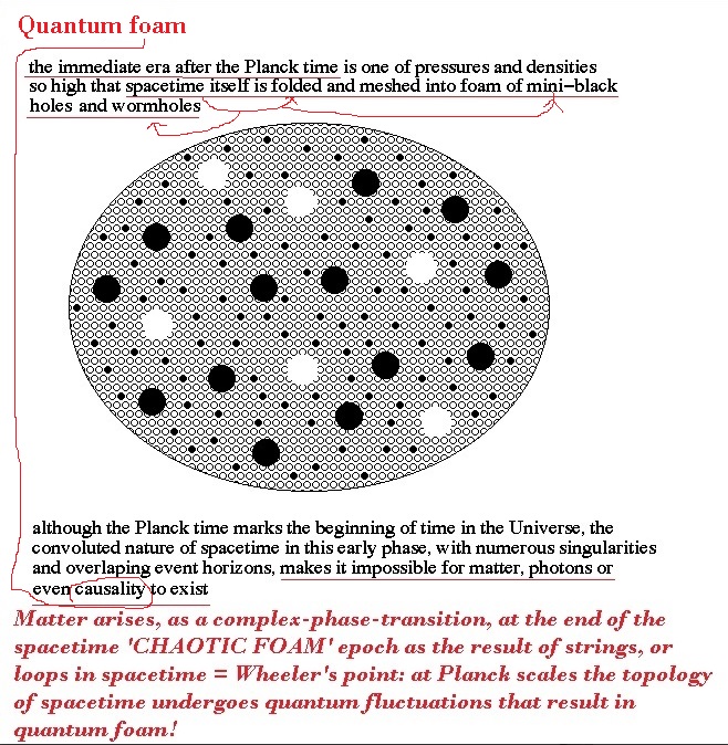
Credit-address for the header photo. In this post, I will discuss and use non-linear multigravity theory to model quantum foam and probe solutions to the cosmological constant cosmic/Planck-scales ‘discrepancy paradox’, related to the hierarchy problem: namely, the 10-47GeV 4/EZP E ≈ 1071GeV cut-off one. Note first that spacetime/quantum randomness-foamy-chaos can be interpreted as a large N composition of Schwarzschild wormholes with a scalar curvature  in n-dimensions being
with  the Regge-Wheeler hypersurface and let me begin with the action involving N massless gravitons without matter fields
with  and
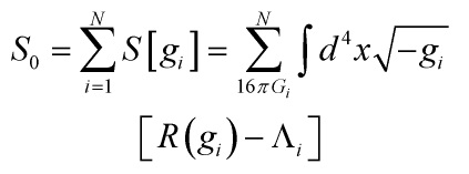
and  being the cosmological constant and the Newton constant corresponding to the i-th universe, respectively, and the total action takes the following form
![\[{S_{tot}} = \sum\limits_{i = 1}^N {S\left[ {{g_i}} \right]} + \lambda {S_{{\mathop{\rm int}} }}\left( {{g_1},...,{g_N}} \right)\]](https://www.georgeshiber.com/wp-content/ql-cache/quicklatex.com-68fb7ce9515f1f4e607267c93ebeae45_l3.png "Rendered by QuickLaTeX.com")
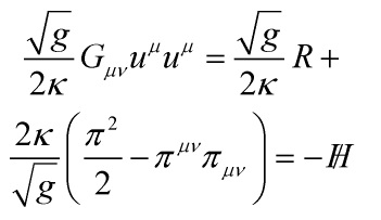
In this way, the action  describes a Bose-Einstein condensates of gravitons. Start with the N = 1 Einstein field equations
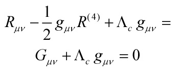
with  the Einstein tensor and injecting a time-like unit vector
  such that
  yields
![\[{G_{\mu \nu }}{u^\mu }{u^\mu } = {\Lambda _c}\]](https://www.georgeshiber.com/wp-content/ql-cache/quicklatex.com-aa1da44f59715b1f224a236a58ccf17f_l3.png "Rendered by QuickLaTeX.com")
which is the Hamiltonian constraint expressed in terms of the equation of motion. So far, we are at the classical ‘level’. The discrepancy between the observed classically-regimed cosmological constant and the quantum-numerical result is in its quantum version: that is, one can derive the expectation value
![\[\left\langle {{\Lambda _c}} \right\rangle \]](https://www.georgeshiber.com/wp-content/ql-cache/quicklatex.com-46a1e8d1074d2036d0f7d87982e15309_l3.png "Rendered by QuickLaTeX.com")
and given that
dimensional analysis for 3-D gives us
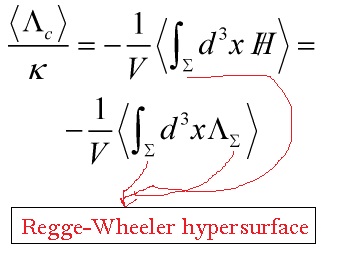
with the r.h.s. equal to

A
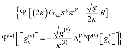
and we integrated over the Regge-Wheeler hypersurface and divided by its volume, and it can be derived starting with the Wheeler-De Witt equation which represents invariance under time reparametrization: that is the Sturm-Liouville cosmological constant problem
The boundary conditions are given by the choice of the quantum fluctuational Gaussian wavefunctionals. Extracting the TT tensor, second order in perturbation, contribution from A, of the spatial part of the metric into a background term,  and a perturbation,
  , yields
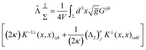
B
with  the inverse DeWitt metric and with the following definition
![\[{K^ \bot }{\left( {\vec x,\vec y} \right)_{iakl}} = \sum\limits_\tau {\frac{{h_{ia}^{(\tau ) \bot }(\vec x)h_{kl}^{(\tau ) \bot }(\vec y)}}{{2\lambda (\tau )}}} \]](https://www.georgeshiber.com/wp-content/ql-cache/quicklatex.com-a0f6976396787afc0a08efdfa5d895b9_l3.png "Rendered by QuickLaTeX.com")
for the propagator
![\[{K^ \bot }{\left( {x,x} \right)_{iakl}}\]](https://www.georgeshiber.com/wp-content/ql-cache/quicklatex.com-f56b58d4771e159ed7fd5229427a8342_l3.png "Rendered by QuickLaTeX.com")
with  the eigenfunctions of
  .
.
Now, the expectation value of  is obtained by inserting the form of the propagator into A and minimizing with respect to the variational function
  . So, the total one loop energy density for TT tensors is
![\[\frac{\Lambda }{{8\pi G}} = - \frac{1}{{4V}}\sum\limits_\tau {\left[ {\sqrt {\omega _1^2\left( \tau \right)} + \sqrt {\omega _2^3\left( \tau \right)} } \right]} \]](https://www.georgeshiber.com/wp-content/ql-cache/quicklatex.com-f680a7c0cac49493d2363aaedc6e7de0_l3.png "Rendered by QuickLaTeX.com")
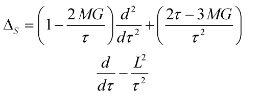
and its contribution to the spin-two operator for the Schwarzschild metric is
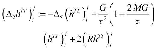
and  is the scalar curved Laplacian, given by
with
![\[R_i^a = \left\{ { - \frac{{2MG}}{{{\tau ^3}}},\frac{{MG}}{{{\tau ^3}}},\frac{{MG}}{{{\tau ^3}}}} \right\}\]](https://www.georgeshiber.com/wp-content/ql-cache/quicklatex.com-108e8c6073d0e7d0f5cb0a1f518ca983_l3.png "Rendered by QuickLaTeX.com")
the mixed Ricci tensor
hence, the scalar curvature is traceless
Thus, we must analyse the eigenvalue equation
![\[\left( {{\Delta _2}{h^{TT}}} \right)_i^j = {\omega ^2}h_j^i\]](https://www.georgeshiber.com/wp-content/ql-cache/quicklatex.com-327282d6d86cba33a106d8d40c54481f_l3.png "Rendered by QuickLaTeX.com")
 the eigenvalue of the corresponding equation. Following Regge-Wheeler, the 3-D gravitational perturbation is represented by its even-parity form
![\[\left( {{h^{even}}} \right)_j^i\left( {\tau ,\vartheta ,\phi } \right) = {\rm{diag}}\left[ {\not H(\tau ),K(\tau ),L(\tau )} \right]{\Upsilon _{lm}}\left( {\vartheta ,\phi } \right)\]](https://www.georgeshiber.com/wp-content/ql-cache/quicklatex.com-50d71c8e88d63bd5bb684e32d117dc65_l3.png "Rendered by QuickLaTeX.com")
Hence, the system
from the throat of the bridge, becomes
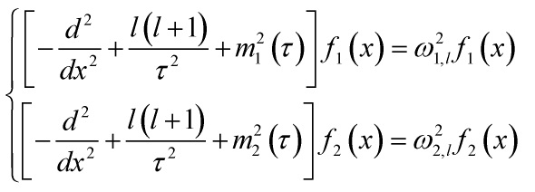
Hence, we have, for  and
and
![\[\left\{ {\begin{array}{*{20}{c}}{m_1^2\left( \tau \right) = {U_1}\left( \tau \right) = m_1^2\left( {\tau ,M} \right) - m_2^2\left( {\tau ,M} \right)}\\{m_2^2\left( \tau \right) = {U_2}\left( \tau \right) = m_1^2\left( {\tau ,M} \right) + m_2^2\left( {\tau ,M} \right)}\end{array}} \right.\]](https://www.georgeshiber.com/wp-content/ql-cache/quicklatex.com-22dbd2587d2dbde9b1e30bedde5b4f4e_l3.png "Rendered by QuickLaTeX.com")
and
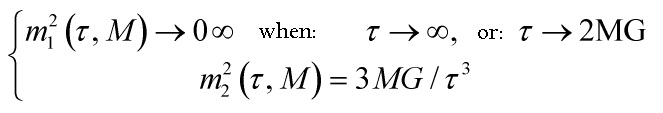
So, one can write
![\[\left\{ {\begin{array}{*{20}{c}}{m_1^2\left( \tau \right) \simeq - \,m_2^2\left( {{\tau _0},M} \right)}\\{m_2^2\left( \tau \right) \simeq + \,m_2^2\left( {{\tau _0},M} \right)}\end{array}} \right.\]](https://www.georgeshiber.com/wp-content/ql-cache/quicklatex.com-4f62e01aabe2999f21df236bd973349c_l3.png "Rendered by QuickLaTeX.com")
where we have
![\[\left\{ {\begin{array}{*{20}{c}}{{\tau _0} > 2MG}\\{m_0^2\left( {{\tau _0},M} \right) = 3MG/\tau _0^3}\end{array}} \right.\]](https://www.georgeshiber.com/wp-content/ql-cache/quicklatex.com-63e9052f97977645b3060ac44841dd81_l3.png "Rendered by QuickLaTeX.com")
We can now explicitly evaluate:
in terms of the effective mass. Via the ‘t Hooft BWM method, one can derive
![\[\begin{array}{c}{\rho _i}\left( \varepsilon \right) = \frac{{m_i^4\left( \tau \right)}}{{256{\pi ^2}}}\left[ {\frac{1}{\varepsilon } + {\rm{In}}\left( {\frac{{{\mu ^2}}}{{m_i^2\left( \tau \right)}}} \right) + 2\,{\rm{In}}\,2 - \frac{1}{2}} \right]\\i = 1,2\end{array}\]](https://www.georgeshiber.com/wp-content/ql-cache/quicklatex.com-ba99cad4870b2b3040d9a87d4c57c10c_l3.png "Rendered by QuickLaTeX.com")
by using the zeta function regularization method to numerically analyse the energy densities  and by introducing the mass parameter
  so as to restore the correct dimension for the regularized quantities. So the energy density is renormalized due to the absorption divergences, yielding the classical constant

removing the dependence on the mass scale , it is appropriate to use the renormalization group equation, which means imposing:
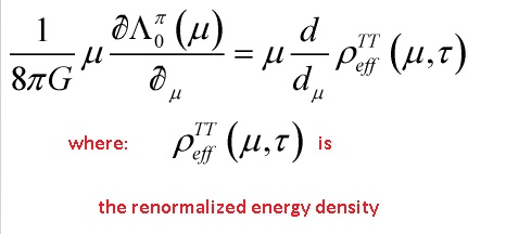
After solving, one realizes that the renormalized constant  should be treated as a running one

and the cosmological constant takes the form
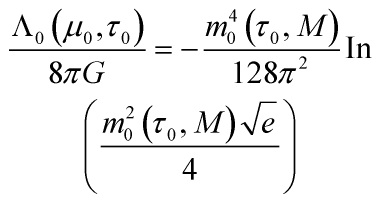
with a minimum
![\[\frac{{m_0^2\left( {{\tau _0},M} \right)\sqrt e }}{{4\mu _0^2}} = \frac{1}{{\sqrt e }}\]](https://www.georgeshiber.com/wp-content/ql-cache/quicklatex.com-7af168f521cc5339de641f4d9f0b2509_l3.png "Rendered by QuickLaTeX.com")
and the condition
![\[\frac{{{\Lambda _0}\left( {{\mu _0},\tau } \right)}}{{8\pi G}} = - \frac{{\mu _0^4}}{{16{e^2}{\pi ^2}}}\]](https://www.georgeshiber.com/wp-content/ql-cache/quicklatex.com-7457ddcd780333e61e7c89642d7379b8_l3.png "Rendered by QuickLaTeX.com")
We are finally in a position to discuss non-linear multigravity gas. For every gravitational field, associate the variables  with the gauge
![\[N_i^{\left( k \right)} = 0\;,\quad \left( {k = 1...{N_w}} \right)\]](https://www.georgeshiber.com/wp-content/ql-cache/quicklatex.com-d46c8747c890fd874d8b1b325db7444b_l3.png "Rendered by QuickLaTeX.com")
and introduce the domain 
and a covering  such that
![\[\begin{array}{c}{\Sigma ^c} = \cup _{k = 1}^{{N_w}}\Sigma _k^c\;,\quad \Sigma _k^c \cap \Sigma _j^c = \emptyset \\k \ne j\end{array}\]](https://www.georgeshiber.com/wp-content/ql-cache/quicklatex.com-4f40e0944df23f613fa26f072cb3a83c_l3.png "Rendered by QuickLaTeX.com")
gives us
Hence, every  has the topology of
  ,
,
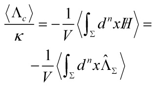
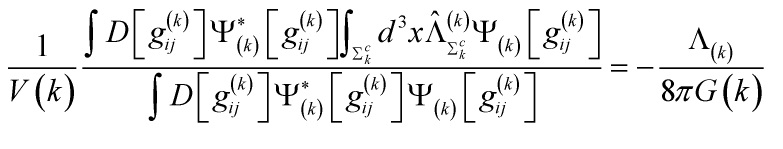
and so the whole physical space containing the energy density will be composed by the non overlapping spaces , yielding a model which is composed by  copies of the same world. Therefore, the final evaluation of the global cosmological constant can be written as
containing the energy density will be composed by the non overlapping spaces , yielding a model which is composed by copies of the same world. Therefore, the final evaluation of the global cosmological constant can be written as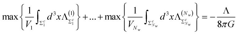
with  the eigenvalue on each , giving us the massive graviton relation
![\[{S_m} = \frac{{m_g^2}}{{8\kappa }}\int {{d^4}} x\sqrt { - \hat g} \left[ {{h^{ij}}{h_{ij}}} \right]\]](https://www.georgeshiber.com/wp-content/ql-cache/quicklatex.com-a843531c0c0380ed559088e948c1cf0e_l3.png "Rendered by QuickLaTeX.com")
which together with
bridges, and thus (partially) solves, the discrepancy paradox. To be continued.
