Continuing from where I left off revealing paradoxical aspects of wave-function collapse involving time-reversal symmetry and the quantum entanglement of the total system consisting of ‘S’, ‘m’ and the quantum-time measuring clock ‘c’ subject to Heisenberg’s UP, consider the collapse equation:
![\[\begin{array}{*{20}{l}}{d{\psi _t}^{S,m,c} = \left[ { - iHdt + \sum\limits_{k = 1}^n {\left( {{L_k} - {\ell _{k,t}}} \right)} } \right.}\\{d{W_{k,t}} - \frac{1}{2}\sum\limits_{k = 1}^n {\left. {\left( {L_k^\dagger {L_k} - 2{\ell _{k,t}}{L_k} + {{\left| {{\ell _{k,t}}} \right|}^2}} \right)} \right]} }\\{{\psi _t}^{S,m,c}}\end{array}\]](https://www.georgeshiber.com/wp-content/ql-cache/quicklatex.com-1a83933a29c2181918c761122e6c8710_l3.png "Rendered by QuickLaTeX.com")
with  the Hilbert-space Lindblad collapse operators,
  given by:
![\[{\ell _{k,t}} \equiv \frac{1}{2}\left\langle {{\psi _t},\left( {L_k^\dagger + {L_k}} \right){\psi _t}^{S,m,c}} \right\rangle \]](https://www.georgeshiber.com/wp-content/ql-cache/quicklatex.com-a5a14b928e977d999181ccfdbdce9f60_l3.png "Rendered by QuickLaTeX.com")
and the first term on the right-hand side represents the unitary quantum evolution, the rest the collapse of the wave-function. Dynamically, to ensure the positivity of the reduced density matrix:
![\[\forall t\left\langle {\left. \psi \right|{{\hat \rho }_S}(t)\left| \psi \right.} \right\rangle \ge 0\]](https://www.georgeshiber.com/wp-content/ql-cache/quicklatex.com-7270119fff2bf743c60271f2653d3f0a_l3.png "Rendered by QuickLaTeX.com")
the Lindblad collapse equation:
![\[\begin{array}{*{20}{l}}{d\left| {{\psi _t}^{S,m,c}} \right\rangle = \left[ { - \frac{i}{\hbar }} \right.Hdt + \sqrt \lambda \int {{d^3}} x\left( {N(\bar x) - {{\left\langle {N(\bar x)} \right\rangle }_t}} \right)}\\{d{W_t}(\bar x) - \frac{\lambda }{2}\int {{d^3}} x\left. {{{\left( {N(\bar x) - {{\left\langle {N(\bar x)} \right\rangle }_t}} \right)}^2}dt} \right]\left| {{\psi _t}^{S,m,c}} \right\rangle }\end{array}\]](https://www.georgeshiber.com/wp-content/ql-cache/quicklatex.com-f089a61dd392ed76a116681960c0ba6e_l3.png "Rendered by QuickLaTeX.com")
would entail that the Lindblad quantum-jump equation:
![\[\begin{array}{l}{\rm{d}}\hat \rho _S^C = - i\left[ {{{\hat H}_S},\hat \rho _S^C} \right]{\rm{d}}t - \\\frac{1}{2}\sum\limits_\mu {{\kappa _\mu }} \left[ {{{\hat L}_\mu },\left[ {{{\hat L}_\mu },\hat \rho _S^C} \right]} \right]{\rm{d}}t + \\\sum\limits_\mu {\sqrt {{\kappa _\mu }} } W\left[ {{{\hat L}_\mu }} \right]\hat \rho _S^C{\rm{d}}{W_\mu }\end{array}\]](https://www.georgeshiber.com/wp-content/ql-cache/quicklatex.com-ee87490921747ac619bc820689a9b67a_l3.png "Rendered by QuickLaTeX.com")
is solvable iff commutes with the position-operator, with:
![\[\begin{array}{l}W\left[ {\hat L} \right]\hat \rho \equiv \hat L\hat \rho + \hat \rho {{\hat L}^\dagger } - \\\hat \rho {\rm{Tr}}\left\{ {\hat L\hat \rho + \hat \rho {{\hat L}^\dagger }} \right\}\end{array}\]](https://www.georgeshiber.com/wp-content/ql-cache/quicklatex.com-ce95b689b7da81151afd2ddb7cc775b3_l3.png "Rendered by QuickLaTeX.com")
where  is the the Markovian reduced density operator, and
  the Weiner-quantum-increments.
However:
![\[\tilde U: = - \frac{\lambda }{2}\int {{d^3}} x{\left( {N(\bar x) - {{\left\langle {N(\bar x)} \right\rangle }_t}} \right)^2}dt(...)\]](https://www.georgeshiber.com/wp-content/ql-cache/quicklatex.com-8da9af8d1ef1c94643c3df2fa7c3a1aa_l3.png "Rendered by QuickLaTeX.com")
commutes with the energy operator. By the Heisenberg energy-time uncertainty principle, the collapse equation cannot be integrated to get the collapse-localization double-integral in 4-D:
![\[{\int {\int {\left| {\Psi _{{t_4}}^I\left( {x,X} \right) + \Psi _{{t_4}}^{II}\left( {x,X} \right)} \right|} } ^2}dxdX = 1\]](https://www.georgeshiber.com/wp-content/ql-cache/quicklatex.com-2f25329efdb1a04f14439fb71d0a3d7a_l3.png "Rendered by QuickLaTeX.com")
Now applying the wave-particle duality to:
![\[\int { - \frac{\lambda }{2}} {d^3}xd{W_t}(\bar x) + \int {\frac{i}{\hbar }Hdt + \sqrt \lambda \int {{d^3}} xd{W_t}(\bar x)} \]](https://www.georgeshiber.com/wp-content/ql-cache/quicklatex.com-4801a59692c5a93dbc1c3f20f40bde0d_l3.png "Rendered by QuickLaTeX.com")
implies therefore, by the time-local non-Markovian master equation:
![\[\frac{{\rm{d}}}{{{\rm{d}}t}}{\hat \rho _S}(t) = \hat K(t){\hat \rho _S}(t)\]](https://www.georgeshiber.com/wp-content/ql-cache/quicklatex.com-5e407999f1779f7470b5710a06ade3df_l3.png "Rendered by QuickLaTeX.com")
that the Lindblad quantum-jump equation is ill-defined over any quantum state describing the total system: in particular, a quantum-time measuring clock (QTMC). This much is guaranteed by the Heisenberg uncertainty principle relating time and energy. Thus, since such a QTMC is essential for Schrödinger’s equation, the paradox is now clear.
Let us look at how quantum Markovian jumps can offer a decoherence way out. Let a system S be described by the master equation for the reduced density operator in the Markovian approximation:
![\[\begin{array}{c}\dot \rho = i\left[ {\hat H,\rho } \right] + \sum\limits_m {{{\hat L}_m}} \hat L_m^\dagger - \frac{1}{2}\hat L_m^\dagger {{\hat L}_m}\rho \\ - \frac{1}{2}\rho \hat L_m^\dagger {{\hat L}_m}\end{array}\]](https://www.georgeshiber.com/wp-content/ql-cache/quicklatex.com-29f800ed3ba0e5b71e45fbb966a689e6_l3.png "Rendered by QuickLaTeX.com")
which has a Heisenberg-cut unraveling into a quantum jump process for pure states, with the usual Hamiltonian and the Lindblad operators which describe the effects of the environment are the set  . Here, I am describing quantum systems via an exhaustive set of possible histories that satisfy a decoherence or consistency-histories criterion obeying the classical probability sum rules. Moreover, such quantum jumps are interpreted as yielding the values of continuous measurements and the histories correspond to records of a classical measuring device that must decohere. Hence, there is a set of decoherent histories that correspond to the quantum trajectories of a continuously measured system. See Ian Percival as well as Lajos Diósi for such remarkable correspondences.
Now take a quantum system with a Hamiltonian  with complete single channel of decay tracked by an external photon detector described by a model of a single 2-level system with states
  and
and  strongly coupled to an environment representing the remaining degrees of freedom. The two crucial properties are clearly, 1) dissipation: Excitations of the states absorbed by the measuring device with a rate
  , with the time-resolution of the detector given by
  , and 2) decoherence: As output mode states become correlated with the internal degrees of freedom of the measuring device, the phase coherence between the ground and excited states of the output mode is completely and tracelessly lost,
and the loss of coherence is far quicker than the actual rate of energy loss, with decoherence rate 
So, the linearized system coupled to the output mode via the Hamiltonian:
![\[{\hat H_I} = \kappa \left( {{{\hat a}^\dagger } \otimes \hat b + \hat a \otimes {{\hat b}^\dagger }} \right)\]](https://www.georgeshiber.com/wp-content/ql-cache/quicklatex.com-19a3d39651d127028a20c2b8ff5313a2_l3.png "Rendered by QuickLaTeX.com")
with the following total Hamiltonian:
![\[\hat H = {\hat H_0} \otimes \hat 1 + \kappa \left( {{{\hat a}^\dagger } \otimes \hat b + \hat a \otimes {{\hat b}^\dagger }} \right)\]](https://www.georgeshiber.com/wp-content/ql-cache/quicklatex.com-10f9b83da2181e2187c255277ed56185_l3.png "Rendered by QuickLaTeX.com")
with  the lowering/raising operators for the system and output mode respectively entails that the total system satisfies the master equation:
![\[\begin{array}{c}\dot \rho = - i\left[ {\hat H,\rho } \right] + {\Gamma _1}\hat b\rho {{\hat b}^\dagger } - \frac{{{\Gamma _1}}}{2}{{\hat b}^\dagger }\hat b\rho \\ - \frac{{{\Gamma _1}}}{2}\rho {{\hat b}^\dagger }\hat b + {\Gamma _2}{\sigma _z}\rho {\sigma _z} - {\Gamma _2}\rho \\ \equiv L_s^L\rho \end{array}\]](https://www.georgeshiber.com/wp-content/ql-cache/quicklatex.com-cc3758ebaace5c12297a8b89dc8bcc3f_l3.png "Rendered by QuickLaTeX.com")
where the Pauli operator  acts on the output mode and
  is the Liouville superoperator. Given that it is a linear equation, it has a solution given as:
![\[\rho ({t_2}) = \exp \left\{ {L_s^L\left( {{t_2} - {t_1}} \right)} \right\}\rho ({t_1})\]](https://www.georgeshiber.com/wp-content/ql-cache/quicklatex.com-f1a8466e72e485c34ff22bc73a776566_l3.png "Rendered by QuickLaTeX.com")
Start with a pure state:
![\[\left| \Psi \right\rangle = \left| \psi \right\rangle \otimes \left| 0 \right\rangle \]](https://www.georgeshiber.com/wp-content/ql-cache/quicklatex.com-09e051db22a432b5d681e2ddba2a2093_l3.png "Rendered by QuickLaTeX.com")
and expand as:
![\[\begin{array}{l}\rho (t) = {\rho _{00}}(t) \otimes \left| 0 \right\rangle \left\langle 0 \right| + {\rho _{01}}(t)\\ \otimes \left| 0 \right\rangle \left\langle 1 \right| + {\rho _{10}}(t) \otimes \left| 1 \right\rangle \left\langle 0 \right| + {\rho _{11}}(t)\\ \otimes \left| 1 \right\rangle \left\langle 1 \right|\end{array}\]](https://www.georgeshiber.com/wp-content/ql-cache/quicklatex.com-be477481984ca97258ff3dc5d8e86626_l3.png "Rendered by QuickLaTeX.com")
So the master equation reduces component-wise to:
![\[\begin{array}{c}{{\dot \rho }_{00}} = - \left[ {\hat H,{\rho _{00}}} \right] - i\kappa {{\hat a}^\dagger }{\rho _{10}} + i\kappa {\rho _{01}}\hat a\\ + {\Gamma _1}{\rho _{11}}\end{array}\]](https://www.georgeshiber.com/wp-content/ql-cache/quicklatex.com-4584090feb53132b2812d5ca794d18c3_l3.png "Rendered by QuickLaTeX.com")
![\[\begin{array}{l}{{\dot \rho }_{01}} = - \left[ {\hat H,{\rho _{01}}} \right] - i\kappa {{\hat a}^\dagger }{\rho _{11}} + i\kappa {\rho _{00}}{{\hat a}^\dagger }\\ - G{\rho _{01}} = \dot \rho _{10}^\dagger \end{array}\]](https://www.georgeshiber.com/wp-content/ql-cache/quicklatex.com-3c059562941350d2d03f665e4852a4c2_l3.png "Rendered by QuickLaTeX.com")
and
![\[\begin{array}{c}{{\dot \rho }_{11}} = - \left[ {\hat H,{\rho _{11}}} \right] - i\kappa \hat a{\rho _{10}} + i\kappa {\rho _{10}}{{\hat a}^\dagger }\\ - {\Gamma _1}{\rho _{11}}\end{array}\]](https://www.georgeshiber.com/wp-content/ql-cache/quicklatex.com-d140d6bd4fa2fb8a99347ba92376b33d_l3.png "Rendered by QuickLaTeX.com")
with:
![\[G = {\Gamma _1}/2 + 2{\Gamma _2} \gg {\Gamma _1} \gg \kappa \]](https://www.georgeshiber.com/wp-content/ql-cache/quicklatex.com-c10e53a07a942000b338ead33dfa3927_l3.png "Rendered by QuickLaTeX.com")
Now, given that the  components are heavily damped, one can adiabatically eliminate all except
  :
:
![\[\begin{array}{l}{{\dot \rho }_{00}} = - i\left[ {{{\hat H}_0},{\rho _{00}}} \right] + \frac{{2{\kappa ^2}}}{G}\hat a{\rho _{00}}{{\hat a}^\dagger }\\ - \frac{{{\kappa ^2}}}{G}{{\hat a}^\dagger }\hat a{\rho _{00}} - \frac{{{\kappa ^2}}}{G}{\rho _{00}}{{\hat a}^\dagger }\hat a\end{array}\]](https://www.georgeshiber.com/wp-content/ql-cache/quicklatex.com-2592efca0fac269fba36c3a766a73687_l3.png "Rendered by QuickLaTeX.com")
Such a master equation can be fleshed out as a sum over quantum jump trajectories. So, let us define a non-Hermitian effective Hamiltonian:
![\[{\hat H_{eff}} = {\hat H_0} - i\left( {{\kappa ^2}/G} \right){\hat a^\dagger }\hat a\]](https://www.georgeshiber.com/wp-content/ql-cache/quicklatex.com-1a16641545b510c8474a518897d4297e_l3.png "Rendered by QuickLaTeX.com")
Hence,  evolves according to the Schrödinger equation:
![\[\frac{{d\left| {\psi _t^{S,m,c}} \right\rangle }}{{dt}} = - \frac{i}{\hbar }{\hat H_{eff}}\left| {\psi _t^{S,m,c}} \right\rangle \]](https://www.georgeshiber.com/wp-content/ql-cache/quicklatex.com-dc22994ac2ae41410b54489844bc5702_l3.png "Rendered by QuickLaTeX.com")
with interruptions at random times by sudden quantum jumps:
![\[\left| {\psi _t^{S,m,c}} \right\rangle \to \hat a\left| {\psi _t^{S,m,c}} \right\rangle \]](https://www.georgeshiber.com/wp-content/ql-cache/quicklatex.com-9e3e8aed7ec3852837892bd13166bfdf_l3.png "Rendered by QuickLaTeX.com")
that correspond to informational detection of photons.
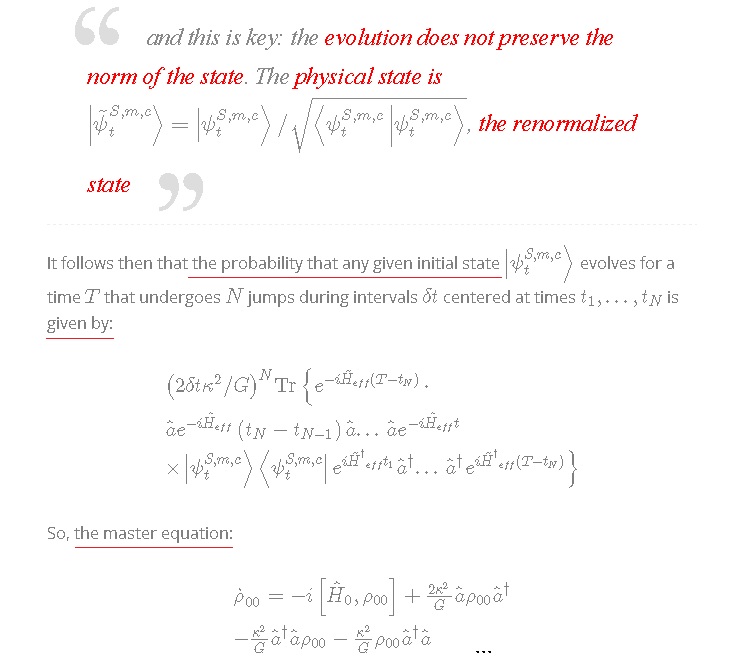
and this is key: the evolution does not preserve the norm of the state. The physical state is  , the renormalized state
, the renormalized stateIt follows then that the probability that any given initial state  evolves for a time
  that undergoes
  jumps during intervals
  centered at times
  is given by:
![\[\begin{array}{l}{\left( {2\delta t{\kappa ^2}/G} \right)^N}{\rm{Tr}}\left\{ {{e^{ - i{{\tilde H}_{eff}}\left( {T - {t_N}} \right)}}} \right. \cdot \\\hat a{e^{ - i{{\hat H}_{eff}}}}\left( {{t_N} - {t_{N - 1}}} \right)\hat a...\,\hat a{e^{ - i{{\hat H}_{eff}}t}}\\ \times \left| {\psi _t^{S,m,c}} \right\rangle \left\langle {\psi _t^{S,m,c}} \right|{e^{i{{\tilde H}^\dagger }_{eff}{t_1}}}{{\hat a}^\dagger }...\,\left. {{{\hat a}^\dagger }{e^{i{{\tilde H}^\dagger }_{eff}\left( {T - {t_N}} \right)}}} \right\}\end{array}\]](https://www.georgeshiber.com/wp-content/ql-cache/quicklatex.com-3f372d7bd33398bf84d97f2a72a11170_l3.png "Rendered by QuickLaTeX.com")
So, the master equation:
is valid iff the Markovian approximation is faithful and valid only on time-scales longer than , hence the jump occurs during an interval  centered on
  .
.
Now, by taking the average of  over all possible trajectories with the probability measure:
the unraveling reproduces the master equation:
let us consider now the decoherent histories picture
A set of decoherent histories for a system is given by choosing a complete set of projections:
![\[\left\{ {\hat P_{{\alpha _j}}^j({t_j})} \right\}\]](https://www.georgeshiber.com/wp-content/ql-cache/quicklatex.com-1685d24360df6744d0f207ceea8202ec_l3.png "Rendered by QuickLaTeX.com")
at a sequence of times  representing exclusively different alternatives histories:
![\[\left\{ {\begin{array}{*{20}{c}}{\sum\limits_{{\alpha _j}} {\hat P_{{\alpha _j}}^j\left( {{t_j}} \right) = \hat 1} }\\{\hat P_{{\alpha _j}}^j\left( {{t_j}} \right)\hat P_{{{\alpha '}_j}}^j\left( {{t_j}} \right) = {\delta _{{\alpha _j}{{\alpha '}_j}}}\hat P_{{\alpha _j}}^j\left( {{t_j}} \right)}\end{array}} \right.\]](https://www.georgeshiber.com/wp-content/ql-cache/quicklatex.com-9334403cd84861c67991da11df12e8b6_l3.png "Rendered by QuickLaTeX.com")
A history  is given by picking one
  at each point in time. Then the decoherence functional for a given pair of histories and
  is:
is:
![\[\begin{array}{l}{D^{dec}}\left[ {h,h'} \right] = {\rm{Tr}}\left\{ {\hat P_{{\alpha _N}}^N\left( {{t_N}} \right)...\hat P_{{\alpha _1}}^1} \right.\left( {{t_1}} \right)\\\rho \left( {{t_0}} \right)\hat P_{{{\alpha '}_1}}^1\left( {{t_1}} \right)...\left. {\hat P_{{{\alpha '}_N}}^N} \right\}\end{array}\]](https://www.georgeshiber.com/wp-content/ql-cache/quicklatex.com-72cb63b6a929efc3e09ad4bd7fc1ea62_l3.png "Rendered by QuickLaTeX.com")
and satisfies the decoherence criterion iff the off-diagonal terms vanish, that is:
![\[{D^{dec}}\left[ {h,h'} \right] = 0\;;\quad h \ne h'\]](https://www.georgeshiber.com/wp-content/ql-cache/quicklatex.com-a005a9d7fa359564dfb73f9f3b29a081_l3.png "Rendered by QuickLaTeX.com")
Now take any initial pure state:
![\[\left| \Psi \right\rangle = \left| {\psi _0^{S,m,c}} \right\rangle \otimes \left| 0 \right\rangle \]](https://www.georgeshiber.com/wp-content/ql-cache/quicklatex.com-4ab8647db6b494f33f10ea32ec762a0c_l3.png "Rendered by QuickLaTeX.com")
and take histories composed only of the Schrödinger-projections:
![\[\left\{ {\begin{array}{*{20}{c}}{{{\hat P}_{S,0}} = \hat 1 \otimes \left| 0 \right\rangle \left\langle 0 \right|}\\{{{\hat P}_{S,1}} = \hat 1 \otimes \left| 1 \right\rangle \left\langle 1 \right|}\end{array}} \right.\]](https://www.georgeshiber.com/wp-content/ql-cache/quicklatex.com-cb0c2acc000175aa594275023f185314_l3.png "Rendered by QuickLaTeX.com")
characterizing the absence or presence of an m-photon in the output mode. Schrödinger-projections are spaced -apart, and a history consists of projections representing a total time  . Using the quantum regression theorem, the above decoherence functional reduces to:
![\[\begin{array}{l}{D^{dec}}\left[ {h,h'} \right] = {\rm{Tr}}\left\{ {{{\hat P}_{{\alpha _N}}}} \right.{e^{L_s^L\delta t}}\left( {{{\hat P}_{{\alpha _{N - 1}}}}{e^{L_s^L\delta t}}} \right.\\\left( {...} \right.{e^{L_s^L\delta t}}\left( {{{\hat P}_{{\alpha _1}}}} \right.\left| \Psi \right\rangle \left\langle \Psi \right.\left| {\left. {{{\hat P}_{{\alpha _1}}}} \right)} \right.\left. {...} \right)\left. {{{\hat P}_{{\alpha _N}}}} \right\}\end{array}\]](https://www.georgeshiber.com/wp-content/ql-cache/quicklatex.com-ee8068d65875188cfbacc90b0f8c918a_l3.png "Rendered by QuickLaTeX.com")
and the Liouville time evolution superoperators:
transform pure states into mixed states.
So, from:
and
one can uniquely determine the character of the different histories, and the central regime is in the range:
![\[\frac{1}{G} \ll \delta t \gg \frac{1}{{{\Gamma _1}}}\]](https://www.georgeshiber.com/wp-content/ql-cache/quicklatex.com-9c17007bb369ef9e9aff5d12742dcb62_l3.png "Rendered by QuickLaTeX.com")
Note, the  terms on this time-scale are sufficient to guarantee decoherence and what is crucial is that the terms resolve into individual pure state trajectories: and that is because
the probability of a photon being emitted in any single time-step is small yet any emission implies there is a non-zero probability of absorption on a time scale
The decoherence-effect effectively gives rise to the terms:
![\[\left\{ {\begin{array}{*{20}{c}}{\left( {{\kappa ^2}/G} \right){{\hat a}^\dagger }\hat a{\rho _{00}}}\\{\left( {{\kappa ^2}/G} \right){\rho _{00}}{{\hat a}^\dagger }\hat a}\end{array}} \right.\]](https://www.georgeshiber.com/wp-content/ql-cache/quicklatex.com-ce1425a2bf034db0082d2e82df0f16c9_l3.png "Rendered by QuickLaTeX.com")
in equation:
and are factored in the effective Hamiltonian:
and such terms are fundamental on a time-scale  , unlike
  , which becomes fundamental on a time scale
It is the term:
![\[\left( {2{\kappa ^2}/G} \right)\hat a{\rho _{00}}{\hat a^\dagger }\]](https://www.georgeshiber.com/wp-content/ql-cache/quicklatex.com-d83c85aceaa050c18680fa974cd9b0b1_l3.png "Rendered by QuickLaTeX.com")
that causes pure states to evolve into mixed states in:
One can maintain the purity of the system-state over a full trajectory by picking a time:  .
.
Hence, with:
![\[\rho = {\rho _{00}} \otimes \left| 0 \right\rangle \left\langle 0 \right|\]](https://www.georgeshiber.com/wp-content/ql-cache/quicklatex.com-f8ee076fa61ec8ae3a3fa9e5279837f9_l3.png "Rendered by QuickLaTeX.com")
and after evolving for a time , the state becomes:
![\[\begin{array}{*{20}{l}}{{{\left( {{e^{L_s^L\delta t}}\rho } \right)}_{00}} = {\rho _{00}} - i\left[ {{{\hat H}_0},{\rho _{00}}} \right]\delta t}\\{ - \frac{{{\kappa ^2}}}{G}{{\hat a}^\dagger }\hat a{\rho _{00}}\delta t - \frac{{{\kappa ^2}}}{G}{\rho _{00}}{{\hat a}^\dagger }\hat a\delta t + {\rm{h}}.{\rm{o}}.{\rm{t}}}\\{ \approx {e^{ - i\left( {{{\hat H}_0} - i\left( {{\kappa ^2}/G} \right){{\hat a}^\dagger }\hat a} \right)\delta t}}{\rho _{00}}{e^{i\left( {{{\hat H}_0} + i\left( {{\kappa ^2}/G} \right){{\hat a}^\dagger }\hat a} \right)\delta t}}}\end{array}\]](https://www.georgeshiber.com/wp-content/ql-cache/quicklatex.com-0024936fc607d64f39314d08ab2a7a40_l3.png "Rendered by QuickLaTeX.com")
![\[\begin{array}{l}{\left( {{e^{L_s^L\delta t}}\rho } \right)_{01}} = \frac{{i\kappa }}{G}{\rho _{00}}{{\hat a}^\dagger } + {\rm{h}}{\rm{.o}}{\rm{.t}}{\rm{.}} = \\\left( {{e^{L_s^L\delta t}}\rho } \right)_{10}^\dagger \end{array}\]](https://www.georgeshiber.com/wp-content/ql-cache/quicklatex.com-b8714dcb786a97d04c599f6028e9eeb7_l3.png "Rendered by QuickLaTeX.com")
and
![\[{\left( {{e^{L_s^L\delta t}}\rho } \right)_{11}} = \frac{{2{\kappa ^2}}}{G}\hat a{\rho _{00}}{\hat a^\dagger }\delta t + {\rm{h}}{\rm{.o}}{\rm{.t}}.\]](https://www.georgeshiber.com/wp-content/ql-cache/quicklatex.com-ab924d114c0ed5c1c40506d8f4caeff6_l3.png "Rendered by QuickLaTeX.com")
Thus, the effective Hamiltonian again has two crucial properties. One is the possibility that the excited-mode photon will be absorbed by the measuring device. The second, negligible though, is the possibility that the excited-mode photon will be coherently re-absorbed by the measuring system.
Now, by combining the above three expressions with the projections:
![\[\left\{ {\begin{array}{*{20}{c}}{{{\hat P}_0}}\\{{{\hat P}_1}}\end{array}} \right.\]](https://www.georgeshiber.com/wp-content/ql-cache/quicklatex.com-dfeed6a104a98ec30c311675a6475691_l3.png "Rendered by QuickLaTeX.com")
we can derive the probabilities for all possible histories. Take the history given by an unbroken string of  projections, corresponding to no excited-mode photon being emitted during a time
  .
.
The probability of such a history is the diagonal element of:
Now, expanding the time evolution superoperator using:
and
one can see now that after we get:
![\[\begin{array}{l}{{\hat P}_0}{e^{L_s^L}}\left( {\left| \psi \right\rangle \left\langle \psi \right| \otimes \left| 0 \right\rangle \left\langle 0 \right|} \right){{\hat P}_0} \approx \\\left( {{e^{ - i\left( {{{\hat H}_0} - i\left( {{\kappa ^2}/G} \right){{\hat a}^\dagger }\hat a} \right)\delta t}}\left| \psi \right\rangle \left\langle \psi \right|{e^{i\left( {{{\hat H}_0} + i\left( {{\kappa ^2}/G} \right){{\hat a}^\dagger }\hat a} \right)\delta t}}} \right)\left| 0 \right\rangle \left\langle 0 \right|\end{array}\]](https://www.georgeshiber.com/wp-content/ql-cache/quicklatex.com-112c046e7b6166d5c4f16f1a37214d3b_l3.png "Rendered by QuickLaTeX.com")
Taking the trace after repetitions, one gets:
![\[p(h) \approx {\rm{Tr}}\left\{ {{e^{ - i{{\hat H}_{eff}}N\delta t}}\left| \psi \right\rangle \left\langle \psi \right|{e^{i{{\hat H}^\dagger }_{eff}N\delta t}}} \right\}\]](https://www.georgeshiber.com/wp-content/ql-cache/quicklatex.com-7e69a6e72deefe4d3ea3914aebd1415a_l3.png "Rendered by QuickLaTeX.com")
which is the probability of the quantum jump trajectory when no jumps are detected
Now, let a photon be emitted at time  and with projection
  instead. The corresponding probability is then:
![\[\begin{array}{l}p(h) \approx \left( {2\delta t{\kappa ^2}/G} \right)\\{\rm{Tr}}\left\{ {\hat a{e^{ - i{{\hat H}_{eff}}N\delta t}}\left| \psi \right\rangle \left\langle \psi \right|{e^{i{{\hat H}^\dagger }_{eff}N\delta t}}{{\hat a}^\dagger }} \right\}\end{array}\]](https://www.georgeshiber.com/wp-content/ql-cache/quicklatex.com-d409bd925d134b61a2d5d39960859023_l3.png "Rendered by QuickLaTeX.com")
again, this is the probability of the corresponding quantum jump trajectory
The question then is: what occurs after the output mode has registered as being in the excited state? Two possibilities exist. One is that the output mode drops back to the un-excited state: measuring state absorption, represented by:
![\[\begin{array}{l}{{\hat P}_0}{e^{L_s^L\delta t}}\left( {\left| {\psi '} \right\rangle \left\langle {\psi '} \right| \otimes \left| 1 \right\rangle \left\langle 1 \right|} \right){{\hat P}_0} \approx \\{\Gamma _1}\delta t\left| {\psi '} \right\rangle \left\langle {\psi '} \right| \otimes \left| 0 \right\rangle \left\langle 0 \right|\end{array}\]](https://www.georgeshiber.com/wp-content/ql-cache/quicklatex.com-ea909128cd04c2d9a2c5ff8950bdcbc1_l3.png "Rendered by QuickLaTeX.com")
Or a constant exited state:
![\[\begin{array}{l}{{\hat P}_1}{e^{L_s^L\delta t}}\left( {\left| {\psi '} \right\rangle \left\langle {\psi '} \right| \otimes \left| 1 \right\rangle \left\langle 1 \right|} \right){{\hat P}_1} \approx \\\left( {1 - {\Gamma _1}\delta t} \right){e^{ - i{{\hat H}_{eff}}\delta t}}\left| {\psi '} \right\rangle \left\langle {\psi '} \right|\\{e^{i{{\hat H}^\dagger }_{eff}\delta t}} \otimes \left| 1 \right\rangle \left\langle 1 \right|\end{array}\]](https://www.georgeshiber.com/wp-content/ql-cache/quicklatex.com-db07047f772c6c0c456047c5effaed6a_l3.png "Rendered by QuickLaTeX.com")
So, the output mode has probability 
 per of regressing back to the ground state, while the system state continues to evolve in accordance with the effective Hamiltonian
  .
.
Hence, we have a near-unity probability of the external mode returning to the ground state within a time of order , thus we can sum over all histories in which the photon is absorbed within this time and again this matches the quantum jump trajectories exactly
, thus we can sum over all histories in which the photon is absorbed within this time and again this matches the quantum jump trajectories exactlyGeneralizing, the probability of such histories will be exactly of the form:
To decohere histories, the following must hold, for  :
:
![\[{\left| {\tilde D\left[ {h,h'} \right]} \right|^2} < {\varepsilon ^2}\tilde D\left[ {h,h'} \right] = {\varepsilon ^2}p(h)p(h')\]](https://www.georgeshiber.com/wp-content/ql-cache/quicklatex.com-eb6c2ee929f2926142654a9bb0672355_l3.png "Rendered by QuickLaTeX.com")
for each separate , . Hence, it suffices to analyze two histories which differ at a single time , one with projection , the other ,
which is equivalent to picking out the  and
and  component of
  at that time
and component of at that timearriving at:
![\[\frac{{{{\left| {\tilde D\left[ {h,h'} \right]} \right|}^2}}}{{p(h)p(h')}} \sim \frac{1}{{{{\left( {G\delta t} \right)}^2}}}\]](https://www.georgeshiber.com/wp-content/ql-cache/quicklatex.com-f09562c6431a652bb35cf572ae7b77c4_l3.png "Rendered by QuickLaTeX.com")
with the sum rules given by  .
.
Concluding then, we have demonstrated that continuous measurements are given by the set of quantum jump trajectories corresponding to a set of decoherent histories that reproduces quantum mechanics as a Bayesian theory over Hilbert space with complex ring.

1 Response
The Cosmological Quantum State from Deformation Quantization
Saturday, December 24, 2016[…] as I showed: the Heisenberg equation with respect to the Lindblad collapse operators {ell _{k,t}}: […]