The D=6 string-string duality, crucial for allowing the interchanging of the roles of 4-D spacetime and string-world-sheet loop expansion, entails that there is an equivalence between the K-3 membrane action and the  orbifold action. Here are some thoughts and reflections.
In the bosonic sector, the membrane action is:
![\[\begin{array}{*{20}{l}}{S = {S_M} + \int_{\partial {M^3}} {\left\{ {\frac{1}{2}} \right.} \left( {{g_{mn}}{\eta ^{ij}} + {b_{mn}}{\varepsilon ^{ij}}} \right)}\\{{\partial _i}{x^m}{\partial _j}{x^n} + \frac{1}{2}\left( {{g_{IJ}}{\eta ^{ij}} + {b_{IJ}}{\varepsilon ^{ij}}} \right)}\\{{\partial _i}{x^I}{\partial _j}{x^J} + {\varepsilon ^{ij}}{\partial _i}{x^J}{\partial _j}{x^m}\left. {A_m^J(x)} \right\}}\end{array}\]](https://www.georgeshiber.com/wp-content/ql-cache/quicklatex.com-4882eceed14877eb1333bb4a24c24503_l3.png "Rendered by QuickLaTeX.com")
where:
![\[\begin{array}{*{20}{l}}{{S_M} = \int_{{M^3}} {\left( {\sqrt { - {g_{mn}}{\partial _i}{x^m}{\partial _j}{x^n}} } \right.} + }\\{\frac{1}{6}{\varepsilon ^{ijk}}{\partial _i}{x^m}{\partial _j}{x^n}{\partial _k}{x^p}\left. {{B_{mnp}}} \right)}\end{array}\]](https://www.georgeshiber.com/wp-content/ql-cache/quicklatex.com-0efe6a7e9fc6909233be8b69d1d9bf82_l3.png "Rendered by QuickLaTeX.com")
Recall I derived the total action:
![\[\begin{array}{l}{S^{Total}} = \frac{1}{{2\pi {\alpha ^\dagger }12}}\int\limits_{{\rm{world - volumes}}} {{d^{26}}} x\,d\,\Omega {\left( {{\phi _{INST}}} \right)^2}\sqrt {\frac{{ - {g_{\mu \nu }}}}{{ - \gamma }}} \,{e^{ - {c_{2n}}/{\Upsilon _\kappa }(\cos \varphi )}} \cdot \\\left( {{R_{icci}} - 4{{\left( {{{\not D}^{SuSy}}\left( {{\phi _{INST}}} \right)} \right)}^2}} \right) + \frac{1}{{12}}H_{3,\mu \nu \lambda }^bH_3^{b,\mu \nu \lambda }/A_\mu ^H + \sum\limits_{D - p - branes} {S_{Dp}^{WV}} \end{array}\]](https://www.georgeshiber.com/wp-content/ql-cache/quicklatex.com-ee1ece1964f54af749ce713bc472b175_l3.png "Rendered by QuickLaTeX.com")
which is highly non-trivial since Clifford algebras are a quantization of exterior algebras. Applying to the Einstein-Minkowski fibre-bundle, we get via Gaussian matrix elimination, an expansion of  via Green’s-functions, yielding the on-shell action of M-theory in the Witten gauge:
![\[\begin{array}{l}{S_M} = \frac{1}{{{k^9}}}\int\limits_{{\rm{world - volumes}}} {{d^{11}}} \sqrt {\frac{{ - {g_{\mu \nu }}}}{{ - \gamma }}} {T_p}^{10}d\Omega {\left( {{\phi _{INST}}} \right)^{26}}\left( {{R_{icci}} - A_\mu ^H\frac{1}{{48}}G_4^2} \right) + \\\sum\limits_{Dp} {D_\mu ^{SuSy}} {e^{ - H_3^b}}/S_{Dp}^{WV} + \sum\limits_{Dp} {D_\nu ^{SuSy}} {e^{H_3^b}}/S_{Dp}^{SV}\end{array}\]](https://www.georgeshiber.com/wp-content/ql-cache/quicklatex.com-1a699b31134d813b59d880d2e5f88662_l3.png "Rendered by QuickLaTeX.com")
with  the kappa symmetry term. With
  the metric on
  , and
, and  the corresponding coordinates with
  an antisymmetric 3-tensor. Hence, the worldvolume
  is:
is:
![\[R \times {S^1} \times {S^1}/{Z_2}\]](https://www.georgeshiber.com/wp-content/ql-cache/quicklatex.com-32cbccc7e51757f72dc1fbc5b9e2a973_l3.png "Rendered by QuickLaTeX.com")
The bosonic sector lives on the boundary of the open membrane: two copies of  , which naturally couple to the U(1) connections
  .
.
Now, double dimensional reduction of the twisted supermembrane on:
![\[{M^{10}} \times {S^1}/{Z_2}\]](https://www.georgeshiber.com/wp-content/ql-cache/quicklatex.com-e24383851b7133382e7efeb5028ec5b8_l3.png "Rendered by QuickLaTeX.com")
of
entails that the bosonic sector is that of the heterotic string:
![\[\begin{array}{*{20}{l}}{{S_h}\int {{d^2}} \sigma \left\{ {\frac{1}{2}} \right.\left( {{g_{mn}}{\eta ^{ij}} + {b_{mn}}{\varepsilon ^{ij}}} \right){\partial _i}{x^m}{\partial _j}{x^n}}\\{ + \frac{1}{2}\left( {{g_{IJ}}{\eta ^{ij}} + {b_{IJ}}{\varepsilon ^{ij}}} \right){\partial _i}{x^I}{\partial _j}{x^I} + }\\{{\varepsilon ^{ij}}{\partial _i}{x^I}{\partial _n}{x^m}\left. {A_m^{(I)}(x)} \right\}}\end{array}\]](https://www.georgeshiber.com/wp-content/ql-cache/quicklatex.com-d29fbffef61d22da311051a09bec0ceb_l3.png "Rendered by QuickLaTeX.com")
with gauge group indices I = 1, … , 16.
It gets interesting when we consider:
![\[{M^{10}} = {T^3}{\rm{ }} \times {\rm{ }}{M^7}\]](https://www.georgeshiber.com/wp-content/ql-cache/quicklatex.com-1490541600394f27d173683be0e42d28_l3.png "Rendered by QuickLaTeX.com")
with dimension:
![\[dim{\rm{ }}{H^1}\left( {{M^7}} \right) = 0\]](https://www.georgeshiber.com/wp-content/ql-cache/quicklatex.com-923dabd7cd3025eb1b80a3d2dccab842_l3.png "Rendered by QuickLaTeX.com")
since the worldsheet action:
![\[{S_{het}} = {S_{st}} + {S_{KK}} + {S_{\bmod }}\]](https://www.georgeshiber.com/wp-content/ql-cache/quicklatex.com-81a754148a2c99518936ae3ed71b4a5e_l3.png "Rendered by QuickLaTeX.com")
is now just a sum of three terms:
![\[{S_{st}} = \int {{d^2}} \sigma \frac{1}{2}\left( {{g_{mn}}{\eta ^{ij}} + {b_{mn}}{\varepsilon ^{ij}}} \right){\partial _i}{x^m}{\partial _j}{x^n}\]](https://www.georgeshiber.com/wp-content/ql-cache/quicklatex.com-0629b1e6eedba3792e43442cb7c8f36c_l3.png "Rendered by QuickLaTeX.com")
![\[{S_{KK}}\int {{d^2}} \sigma {\varepsilon ^{ij}}{\partial _i}{x^I}{\partial _j}{x^m}A_m^I\]](https://www.georgeshiber.com/wp-content/ql-cache/quicklatex.com-321bba037609cead48bbf2d93b34bd6d_l3.png "Rendered by QuickLaTeX.com")
![\[{S_{\,\bmod \,}} = \int {{d^2}} \sigma \frac{1}{2}\left( {{g_{IJ}}{\eta ^{ij}} + {b_{IJ}}{\varepsilon ^{ij}}} \right){\partial _i}{x^J}{\partial _j}{x^I}\]](https://www.georgeshiber.com/wp-content/ql-cache/quicklatex.com-60cffd8d87242328b3552e5b5f9d9b34_l3.png "Rendered by QuickLaTeX.com")
and the index I = 1, … , 22 labels 22 gauge fields: 16 coming from the internal dimensions of the heterotic string, and the other 6 gauge fields are the KK modes of the metric and antisymmetric tensor. The action  has a massless spectrum given by moduli fields corresponding to deformations of the Narain lattice and thus take values in the group manifold:
![\[\frac{{SO\left( {19,3} \right)}}{{SO\left( {19} \right) \times SO\left( 3 \right)}}\]](https://www.georgeshiber.com/wp-content/ql-cache/quicklatex.com-36acfc52490cab43de512dee7ad8cb13_l3.png "Rendered by QuickLaTeX.com")
Now, something fundamentally deep has occurred: all the gauge fields of the action  have appeared within a two-dimensional theory, and not a three-dimensional theory
have appeared within a two-dimensional theory, and not a three-dimensional theoryThis is precisely the long wavelength limit behavior of the open membrane:
the gauge fields are defined in terms of fields which live on 10-dimensional boundaries of M-theory
In the closed membrane case:
the gauge fields are defined in terms of 11-dimensional fields
Hence, the gauge fields of the closed membrane must be defined over M3 and not over its boundary, unlike the closed membrane, whose action on  is:
is:
![\[\begin{array}{*{20}{l}}{{{S'}_M} = \int_{{M^3}} {{d^3}} \zeta \left( {\sqrt { - {g_{mn}}{\partial _i}{x^m}{\partial _j}{x^n}} } \right.}\\{ + \frac{1}{6}{\varepsilon ^{ijk}}{\partial _i}{x^m}{\partial _j}{x^n}\left. {{\partial _k}{x^p}{B_{mnp}}} \right)}\end{array}\]](https://www.georgeshiber.com/wp-content/ql-cache/quicklatex.com-98af6d6565ca659b720c9463c50042c5_l3.png "Rendered by QuickLaTeX.com")
where is  with the spacetime being
  .
.
Hence, the closed membrane action  on reduces to:
![\[{S'_M} = {S'_{st}} + {S'_{KK}} + {S'_{\bmod }}\]](https://www.georgeshiber.com/wp-content/ql-cache/quicklatex.com-04df1e610c82d58dce457d5feddfa1a4_l3.png "Rendered by QuickLaTeX.com")
with:
![\[{S'_{KK}} = \frac{1}{6}\int {{d^3}} \sigma {\varepsilon ^{ijk}}{\partial _i}{x^a}{\partial _j}{x^b}{\partial _k}{x^m}{B_{abm}}\]](https://www.georgeshiber.com/wp-content/ql-cache/quicklatex.com-e5448db90892dcc3e5fb80779683744b_l3.png "Rendered by QuickLaTeX.com")
and
![\[{S'_{\,\bmod \,}} = \int {{d^3}} \sigma \sqrt { - {g_{ab}}{\partial _i}{x^a}{\partial _j}{x^b}} + \frac{1}{6}{\varepsilon ^{ijk}}{\partial _i}{x^a}{\partial _j}{x^b}{\partial _k}{x^c}{B_{abc}}\]](https://www.georgeshiber.com/wp-content/ql-cache/quicklatex.com-0a615f78eff9587909eeeeeb359fce26_l3.png "Rendered by QuickLaTeX.com")
and since  surfaces have no one-cycles, it follows that the three-form potential that appears in
  of the action:
can be expanded in terms of the cocycles of .
For the 22 2-cocycles of , one can decompose  in a similar way for the two-form potential:
![\[{B_{abm}} = b_{ab}^I\left( {{x^a}} \right)C_m^I\left( {{x^r}} \right)\]](https://www.georgeshiber.com/wp-content/ql-cache/quicklatex.com-0447f588074948952c1db4beac60d28e_l3.png "Rendered by QuickLaTeX.com")
with I = 1, …, 22 labeling the two-cycles of . So after insertion into , we can derive:
![\[\int_{{M^3}} {{\varepsilon ^{ijk}}} {\partial _i}{x^m}{\partial _j}{x^b}{\partial _k}{x^a}b_{ab}^I\left( {{x^c}} \right)C_m^I\left( {{x^r}} \right)\]](https://www.georgeshiber.com/wp-content/ql-cache/quicklatex.com-c7f56c58debe8ebc1b43f41bd84d4656_l3.png "Rendered by QuickLaTeX.com")
Applying reparametrization invariance, one can set:
![\[\rho = {x^{11}}\]](https://www.georgeshiber.com/wp-content/ql-cache/quicklatex.com-1f7ec6cd61e0ab7a03139ea3327b1095_l3.png "Rendered by QuickLaTeX.com")
where  is a worldvolume coordinate, and now one performs a dimensional reduction of:
Here are the key propositions relevant to the membrane/string duality of the low energy theory in D=7.
- the kinetic terms for the gauge fields in D=7 supergravity are:
![\[\int_{{M^7}} {\sqrt { - {g^{\left( 7 \right)}}} } {a_{IJ}}F_{mn}^I{F^{Jmn}}\]](https://www.georgeshiber.com/wp-content/ql-cache/quicklatex.com-56e7105734ee1982f1984ab6bf5fbccd_l3.png "Rendered by QuickLaTeX.com")
derived by a split of the 4-4 field strength  , of the 11-dimensional supergravity action:
![\[{H_{abmn}} = b_{ab}^IF_{mn}^I\]](https://www.georgeshiber.com/wp-content/ql-cache/quicklatex.com-72f52351dea137babff99faba57c1fdc_l3.png "Rendered by QuickLaTeX.com")
from the following term:
![\[\begin{array}{l}\int_{{M^{11}}} {\sqrt { - {g^{\left( {11} \right)}}} } {H^2} = \int_{{M^7}} {\sqrt { - {g^{\left( 7 \right)}}} } F_{mn}^I{F^{Jmn}}\\\int_{K3} {\sqrt { - {g^{\left( {K3} \right)}}} } b_{ab}^I{b^{Jab}}\end{array}\]](https://www.georgeshiber.com/wp-content/ql-cache/quicklatex.com-052ac78e37ca1a3b75183eae1c4d9fd0_l3.png "Rendered by QuickLaTeX.com")
- Membrane/string duality in D=7 requires the existence of a point in the moduli space of where all the 22 gauge fields are enhanced via U(1) gauging: this is key to preserving kappa symmetry. Thus, at the point in the moduli space when the 22 two-cycles vanish the following holds:
![\[\left\{ {\begin{array}{*{20}{c}}{{\partial _{{x^{11}}}}b_{ab}^I = 0}\\{{\partial _{{x^{11}}}}g_{ab}^I = 0}\end{array}} \right.\]](https://www.georgeshiber.com/wp-content/ql-cache/quicklatex.com-2b0f4b9d5d77c8bed96b22064e460acf_l3.png "Rendered by QuickLaTeX.com")
- Hence, dimensional reduction yields:
![\[\int_{{M^2}} {{\varepsilon ^{ij}}} {\partial _i}{x^m}{\partial _j}{x^b}b_{11b}^IC_m^I\]](https://www.georgeshiber.com/wp-content/ql-cache/quicklatex.com-1a7f4253267196f7a5558a99f7e2795a_l3.png "Rendered by QuickLaTeX.com")
So, the S-duality map:
![\[\left\{ {\begin{array}{*{20}{c}}{b_{a11}^I{\partial _j}{x^a} \to {\partial _j}{x^I}}\\{C_m^I \to A_m^I}\end{array}} \right.\]](https://www.georgeshiber.com/wp-content/ql-cache/quicklatex.com-e2f9a221061be365440cb1422776de54_l3.png "Rendered by QuickLaTeX.com")
takes:
to:
![\[\int_{{M^2}} {{\varepsilon ^{ij}}} {\partial _i}{x^I}A_m^I\]](https://www.georgeshiber.com/wp-content/ql-cache/quicklatex.com-8f87eaf161ec4f3c7368c91d48fc8fa4_l3.png "Rendered by QuickLaTeX.com")
and is equivalent to the term  in:
in:
So, the above map acts on the induced metric on the worldvolume. It follows then that the term in  in:
in:
yields, after a double dimensional reduction of  , the following:
![\[\int {{d^2}} \sigma \frac{1}{2}\left( {{g_{IJ}}{\eta ^{ij}} + {b_{IJ}}{\varepsilon ^{ij}}} \right){\partial _i}{x^J}{\partial _j}{x^I}\]](https://www.georgeshiber.com/wp-content/ql-cache/quicklatex.com-d3bea1c14f5364da1ef608c65010b765_l3.png "Rendered by QuickLaTeX.com")
with:
![\[\left\{ {\begin{array}{*{20}{c}}{{g_{IJ}} = {g_{ab}}b_I^{11a}b_J^{11b}}\\{{b_{IJ}} = {B_{ab11}}b_I^{11a}b_J^{11b}}\end{array}} \right.\]](https://www.georgeshiber.com/wp-content/ql-cache/quicklatex.com-3c31ccb17e56adf021f62623aa3eacb3_l3.png "Rendered by QuickLaTeX.com")
which yields an equivalence between:
and
Thus, the S-duality map that takes to also takes to the dimensionally reduced .
To achieve the matching of gauge sectors of the closed and open membrane, we must generate the gauge fields of the closed membrane before dimensionally reducing the theory, as opposed to the gauge fields of the open membrane, which are always generated within the two-dimensional theory. This explains the origin of strong-weak duality in string theory. The strong coupling limit of type IIA string is 11-dimensional supergravity which is believed to arise as the long wavelength limit of supermembrane theory. So, gauge fields present in the 3-dimensional theory will be strongly interacting, and will continue to be strongly interacting after dimensional reduction to a two-dimensional theory. However, the open membrane has its gauge fields appearing in two dimensional theories, which are therefore weakly interacting.
So, we must consider the spacetime part of the action for the closed membrane:
The term:
![\[\int_{{M^3}} {\sqrt { - {g_{mn}}{\partial _i}{x^m}{\partial _j}{x^n}} } \]](https://www.georgeshiber.com/wp-content/ql-cache/quicklatex.com-de67cd79d00d327bc828aee6c7de46ac_l3.png "Rendered by QuickLaTeX.com")
can be dimensionally reduced to:
![\[\int_{{M^2}} {\sqrt { - {g_{mn}}{\partial _i}{x^m}{\partial _j}{x^n}} } \]](https://www.georgeshiber.com/wp-content/ql-cache/quicklatex.com-3995bcaf3340358c53a6f520fe0fbdc0_l3.png "Rendered by QuickLaTeX.com")
which is equivalent to the first term in:
and the term:
![\[\int_{{M^3}} {{\varepsilon ^{ijk}}} {\partial _i}{x^m}{\partial _j}{x^n}{\partial _k}{x^p}{B_{pmn}}\]](https://www.georgeshiber.com/wp-content/ql-cache/quicklatex.com-f23dcb80621a3ae7f36fb2916b714d53_l3.png "Rendered by QuickLaTeX.com")
maps to:
![\[\int_W {d{\Sigma ^{mnpq}}} {H_{mnpq}}\]](https://www.georgeshiber.com/wp-content/ql-cache/quicklatex.com-8156f41d2926a8ced468436125cb3f08_l3.png "Rendered by QuickLaTeX.com")
with and  members of
Now, since the term is topological, and S-duality of the seven dimensional space entails:
![\[{H^3}\left( {{M^7}} \right) = {H^4}\left( {{M^7}} \right)\]](https://www.georgeshiber.com/wp-content/ql-cache/quicklatex.com-d9c05015dd9d29f00c9c20d2e513c399_l3.png "Rendered by QuickLaTeX.com")
then one can reduce:
to:
![\[\int_{ * W} {d{\Sigma ^{mnp}}} {H_{mnp}}\]](https://www.georgeshiber.com/wp-content/ql-cache/quicklatex.com-b6c0d1d826f9358d6dfdcd137726e327_l3.png "Rendered by QuickLaTeX.com")
with  the Hodge dual and in turn, allows us to further reduce to:
![\[\int_{{M^2}} {{\varepsilon ^{ij}}} {\partial _i}{x^m}{\partial _j}{x^n}{b_{nm}}\]](https://www.georgeshiber.com/wp-content/ql-cache/quicklatex.com-ae29c005fb36f303b87942a85e3732be_l3.png "Rendered by QuickLaTeX.com")
Therefore the b-term in the spacetime string action is a direct consequence of the duality of the seven dimensional duality between 3- and 4-forms, and so the dimensional reduction of  yields the term
  , and this is tantamount to mapping the closed membrane action on to the open membrane action on , thus D=6 string-string duality follows and both theories will have the same spacetime supersymmetry since they have the same massless spectra
yields the term , and this is tantamount to mapping the closed membrane action on to the open membrane action on , thus D=6 string-string duality follows and both theories will have the same spacetime supersymmetry since they have the same massless spectraThis naturally brings us to the connection between string field theory and Dp-branes. Recall that one derives the string propagator by an evaluation of the Witten super-symmetric quantum path integral on a fiber-strip with the Polyakov string action:
![\[G\left[ {{X_1};{X_2}} \right] = \int {D\left[ h \right]} D\left[ X \right]\exp \left( {iS} \right)\]](https://www.georgeshiber.com/wp-content/ql-cache/quicklatex.com-798fe18248f6089fbf239f15e3dd158c_l3.png "Rendered by QuickLaTeX.com")
with:
![\[S = - \frac{1}{{4\pi \alpha '}}\int_M {d\tau d\sigma } \sqrt { - h} {h^{\alpha \beta }}\frac{{\partial {X^I}}}{{\partial {\sigma ^\alpha }}}\frac{{\partial {X^J}}}{{\partial {\sigma ^\beta }}}{\eta _{IJ}}\]](https://www.georgeshiber.com/wp-content/ql-cache/quicklatex.com-da305c8be1d257dd1323751682e03cd3_l3.png "Rendered by QuickLaTeX.com")
for  and the Regge parameter clear from context. In the proper-time gauge and the normal modes of the lapse and shift function in 2-D, the Polyakov metric has the following property:
![\[\sqrt { - h} {h^{\alpha \beta }} = \frac{1}{{{N_1}}}\left( {\begin{array}{*{20}{c}}{ - 1}&{{N_2}}\\{{N_2}}&{{{\left( {{N_1}} \right)}^2} - {{\left( {{N_2}} \right)}^2}}\end{array}} \right)\]](https://www.georgeshiber.com/wp-content/ql-cache/quicklatex.com-9ae8c45d036885c10dc38e6ff59b5dbd_l3.png "Rendered by QuickLaTeX.com")
allowing us to derive the open string field Polyakov propagator on the Dp-branes:
![\[\begin{array}{c}G\left[ {{X_1};{X_2}} \right) = \int_0^\infty {ds} \left\langle {{X_1}\left| {\exp \left[ { - is\left( {{L_0} - i\tilde \varepsilon } \right)} \right]} \right|{X_2}} \right\rangle \\ = \left\langle {{X_1}\left| {\frac{1}{{{L_0} - i\tilde \varepsilon }}} \right|{X_2}} \right\rangle \end{array}\]](https://www.georgeshiber.com/wp-content/ql-cache/quicklatex.com-89438f647f490708cfa6e25a36fb1a7c_l3.png "Rendered by QuickLaTeX.com")
with:
![\[{L_0} = \frac{{{p^\mu }{p_\mu }}}{2} + \sum\limits_{n = 1} {\frac{1}{2}} \left( {p_n^Ip_n^J + {n^2}x_n^Ix_n^J} \right){\eta _{IJ}} - 1\]](https://www.georgeshiber.com/wp-content/ql-cache/quicklatex.com-6d60fddf6bf43dec74fc87fd21577875_l3.png "Rendered by QuickLaTeX.com")
and the momentum operators are given by:
![\[{P^\mu }\left( \sigma \right) = \frac{1}{\pi }{\left( {{p^\mu } + \sqrt 2 \sum\limits_{n = 1} {p_n^\mu \cos \left( {n\sigma } \right)} } \right)_{,\mu = 0,1,...,d}}\]](https://www.georgeshiber.com/wp-content/ql-cache/quicklatex.com-19aa95d541a432d36912934ee4da0545_l3.png "Rendered by QuickLaTeX.com")
![\[{P^i}\left( \sigma \right) = \frac{{\sqrt 2 }}{\pi }{\sum\limits_{n = 1} {p_n^i\sin \left( {n\sigma } \right)} _{,i = 0,1,...,d}}\]](https://www.georgeshiber.com/wp-content/ql-cache/quicklatex.com-8e20579a7449b7d5bdbff4e53754b083_l3.png "Rendered by QuickLaTeX.com")
Since open string end-points are topologically glued to  Dp-branes, open strings must have
  inequivalent quantum states and thus, the string field
  has to carry the gauge group indices of
  :
:
![\[\Psi \left[ X \right] = \frac{1}{{\sqrt 2 }}{\Psi ^0}\left[ X \right] + {\Psi ^a}\left[ X \right]{T^a}\]](https://www.georgeshiber.com/wp-content/ql-cache/quicklatex.com-c5e27c084525d92f86754729a2d582fc_l3.png "Rendered by QuickLaTeX.com")
where  are the generators of the SU(N) group, with
  . Hence, the string propagator on multi-Dp-branes takes the following form, with contraction and indices ordering:
![\[\begin{array}{l}{G^{ab}}\left[ {{X_1};{X_2}} \right] = i\left\langle {T{\Psi ^a}\left[ {{X_1}} \right]{\Psi ^b}\left[ {{X_2}} \right]} \right\rangle \\ = i\int D \left[ X \right]{\Psi ^a}\left[ {{X_1}} \right]{\Psi ^b}\left[ {{X_2}} \right]\exp \left\{ { - i\int {D\left[ X \right]{\rm{tr}}\Psi \left( {{L_0} + i\tilde \varepsilon } \right)\Psi } } \right\}\end{array}\]](https://www.georgeshiber.com/wp-content/ql-cache/quicklatex.com-bc885ff62f8a5f00226a13c4b93595b2_l3.png "Rendered by QuickLaTeX.com")
which yields the field theory action:
![\[{S_0} = \int {D\left[ X \right]} {\rm{tr}}\Psi \left( {{L_0} - i\tilde \varepsilon } \right)\Psi \]](https://www.georgeshiber.com/wp-content/ql-cache/quicklatex.com-32774ac27766b67c2424ab329e11df4d_l3.png "Rendered by QuickLaTeX.com")
BRST-invariantly as:
![\[{S_0} = \int {{\rm{tr}}\Psi } * Q_{BRST}^{generators}\Psi \]](https://www.georgeshiber.com/wp-content/ql-cache/quicklatex.com-9b3038c73f91afcf152347a5be6cd8af_l3.png "Rendered by QuickLaTeX.com")
Hence, the above field theory action implies that the string-string duality associates to every Dp–Brane a solution corresponding to the d–dimensional string–frame Lagrangian:
![\[\begin{array}{c}{\mathcal{L}_{S,d}} = \sqrt {\left| g \right|} \left\{ {{e^{ - 2\phi }}} \right.\left[ {R - 4{{\left( {\partial \phi } \right)}^2}} \right] + \\\frac{{{{( - )}^{p + 1}}}}{{2\left( {p + 2} \right)!}}{e^{a\phi }}\left. {F_{\left( {p + 2} \right)}^2} \right\}\end{array}\]](https://www.georgeshiber.com/wp-content/ql-cache/quicklatex.com-e595d8bd49324003a7101ba1a1a1a8fb_l3.png "Rendered by QuickLaTeX.com")
with  the dilaton,
  the curvature of a (p + 1)–form gauge field:
![\[{F_{\left( {p + 2} \right)}} = d{A_{\left( {p + 1} \right)}}\]](https://www.georgeshiber.com/wp-content/ql-cache/quicklatex.com-cd0c901de42bb6693fe2801fd4a9f2b0_l3.png "Rendered by QuickLaTeX.com")
where the two–index NS/NS tensor  and the dual six-index heterotic five–brane tensor
  are given by:
![\[S_{WZ}^{(1)} = \int {{d^2}} \xi {B^{(1)}}\]](https://www.georgeshiber.com/wp-content/ql-cache/quicklatex.com-5d8b9edae194db0d7a556ece4fa9f6c1_l3.png "Rendered by QuickLaTeX.com")
and
![\[S_{WZ}^{(5)} = \int {{d^6}} \xi \tilde B_{het}^{(1)}\]](https://www.georgeshiber.com/wp-content/ql-cache/quicklatex.com-5b105c67ef55e788a6d680ffdcb1aa0f_l3.png "Rendered by QuickLaTeX.com")
Now we have the general form of a 10-D p-brane solution:
![\[\left\{ {\begin{array}{*{20}{c}}{ds_{S,d}^2 = {H^\alpha }dx_{\left( {p + 1} \right)}^2 - {H^\beta }dx_{\left( {D - p - 1} \right)}^2}\\{{e^{2\phi }} = {H^\gamma }}\\{{F_{0...pi}} = \delta {\partial _i}{H^{\tilde \varepsilon }}}\end{array}} \right.\]](https://www.georgeshiber.com/wp-content/ql-cache/quicklatex.com-2289bec5801dc6befb29272db1a7515b_l3.png "Rendered by QuickLaTeX.com")
with:
![\[\left\{ {\begin{array}{*{20}{c}}{\alpha = \frac{1}{N}\left( {2 - a} \right)}\\{\beta = - \frac{1}{N}\left( {2 + a} \right)}\end{array}} \right.\]](https://www.georgeshiber.com/wp-content/ql-cache/quicklatex.com-b182b607ad4469d90d42c16b510ad6b1_l3.png "Rendered by QuickLaTeX.com")
and:
![\[\left\{ {\begin{array}{*{20}{c}}{\gamma = \frac{1}{N}\left[ {2\left( {p + 1} \right) + \left( {2 + a} \right)\left( {1 - \frac{1}{2}d} \right)} \right]}\\{{\delta ^2} = - \frac{4}{N},\quad \,\tilde \varepsilon = - 1}\end{array}} \right.\]](https://www.georgeshiber.com/wp-content/ql-cache/quicklatex.com-a044702ce4ba6147ef16eec78b0e1c34_l3.png "Rendered by QuickLaTeX.com")
with
![\[N = \left( {p + 1} \right)a + \left( {1 - \frac{1}{2}d} \right){\left( {1 + \frac{1}{2}a} \right)^2}\]](https://www.georgeshiber.com/wp-content/ql-cache/quicklatex.com-67348340f5803c0b582c76ab4e083b0c_l3.png "Rendered by QuickLaTeX.com")
The general form of 11-D Mp–branes solutions, noting the absence of the dilaton field, with the following Lagrangian:
![\[{\mathcal{L}_{Ein,d}} = \sqrt {\left| g \right|} \left[ {R + \frac{1}{2}{{\left( {\partial \phi } \right)}^2} + \frac{{{{( - )}^{p + 1}}}}{{2\left( {p + 2} \right)!}}{e^{\alpha \phi }}F_{\left( {p + 2} \right)}^2} \right]\]](https://www.georgeshiber.com/wp-content/ql-cache/quicklatex.com-66fe4e93349a0e2c7ade0c36f5b8fb86_l3.png "Rendered by QuickLaTeX.com")
is:
![\[\begin{array}{*{20}{c}}{\alpha = - \frac{4}{N}\left( {d - p - 3} \right),}&{\beta = \frac{4}{N}\left( {p + 1} \right)}\\{\gamma = \frac{{4a}}{N}\left( {d - 2} \right),}&\begin{array}{l}{\delta ^2} = \frac{4}{N}\left( {d - 2} \right)\\\tilde \varepsilon = - 1\end{array}\end{array}\]](https://www.georgeshiber.com/wp-content/ql-cache/quicklatex.com-5a39bda56f1832e2848d86fd66141721_l3.png "Rendered by QuickLaTeX.com")
Hence, the M2-brane solution is:
![\[ds_{Ein,11}^2 = {H^{ - 2/3}}dx_{\left( 3 \right)}^2 - {H^{1/3}}dx_{\left( 8 \right)}^2\]](https://www.georgeshiber.com/wp-content/ql-cache/quicklatex.com-af2a8ff75cc6f20b3bfa0966dbfe56bd_l3.png "Rendered by QuickLaTeX.com")
![\[{F_{012i}} = {\partial _i}{H^{ - 1}}\]](https://www.georgeshiber.com/wp-content/ql-cache/quicklatex.com-4f548887d4bdcec24b1a5cb6c62b8002_l3.png "Rendered by QuickLaTeX.com")
squaring the field strength gives the following M5-brane solution:
![\[ds_{Ein,11}^2 = {H^{ - 1/3}}dx_{\left( 6 \right)}^2 - {H^{2/3}}dx_{\left( 5 \right)}^2\]](https://www.georgeshiber.com/wp-content/ql-cache/quicklatex.com-ad2906fb1b75064bea61b2a955c2a32f_l3.png "Rendered by QuickLaTeX.com")
![\[{F_{012345i}} = {\partial _i}{H^{ - 1}}\]](https://www.georgeshiber.com/wp-content/ql-cache/quicklatex.com-347ea734ef507639f370b94b3e6ed855_l3.png "Rendered by QuickLaTeX.com")
In the string-frame Ramond-Ramond gauge field Lagrangian:
Dp-brane solutions have the following form:
![\[ds_{S,10}^2 = {H^{ - 1/2}}dx_{\left( {p + 1} \right)}^2 - {H^{1/2}}dx_{\left( {9 - p} \right)}^2\]](https://www.georgeshiber.com/wp-content/ql-cache/quicklatex.com-04f51d7d8c33db506ee2eec2b1336ec0_l3.png "Rendered by QuickLaTeX.com")
![\[{e^{2\phi }} = {H^{ - \frac{1}{2}\left( {p - 3} \right)}}\]](https://www.georgeshiber.com/wp-content/ql-cache/quicklatex.com-1f830668c0ea714c70b54e0b881afe1d_l3.png "Rendered by QuickLaTeX.com")
![\[{F_{0...pi}} = {\partial _i}{H^{ - 1}}\]](https://www.georgeshiber.com/wp-content/ql-cache/quicklatex.com-45311ed56ba79961d8f7751080d9815d_l3.png "Rendered by QuickLaTeX.com")
From the string-string duality above and  , we can derive the kinetic term of Dp–branes in terms of the Born–Infeld action with the following form:
![\[{S^{Dp}} = \int {{d^{p + 1}}} \xi {e^{ - \phi }}\sqrt {\left| {\det \left( {{g_{ij}} + {{\tilde F}_{ij}}} \right)} \right|} \]](https://www.georgeshiber.com/wp-content/ql-cache/quicklatex.com-5da9298ee92a4d6d6a2f89ce2bf9f8be_l3.png "Rendered by QuickLaTeX.com")
with the embedding metric and the gauge field world-volume curvature manifest, entailing the existence of a WZ/RR term that couples to Dp-branes:
![\[S_{WZ}^{Dp} = \int {{d^{p + 1}}} \xi \tilde {\rm A}{e^{\tilde F}}\]](https://www.georgeshiber.com/wp-content/ql-cache/quicklatex.com-e66428719be07e30dd2fdaad3d39a249_l3.png "Rendered by QuickLaTeX.com")
![\[\tilde {\rm A} = \sum\nolimits_{q = 0}^9 {{A_{\left( {q + 1} \right)}}} \]](https://www.georgeshiber.com/wp-content/ql-cache/quicklatex.com-676b3af87cdd0048fa2e637b7f334ea8_l3.png "Rendered by QuickLaTeX.com")
and where the heterotic 5–brane, the IIA five–brane and the D5–brane dual potentials are given by:
![\[^ * d{B^{(1)}} = d\tilde B_{het}^{(1)}\]](https://www.georgeshiber.com/wp-content/ql-cache/quicklatex.com-fe6867b4ded1eccac69412545aa940fe_l3.png "Rendered by QuickLaTeX.com")
![\[^ * d{B^{(1)}} = d\tilde B_{{\rm{IIA}}}^{(1)} - \frac{{105}}{4}CdC - 7{A^{(1)}}G\left( {\tilde C} \right)\]](https://www.georgeshiber.com/wp-content/ql-cache/quicklatex.com-85380d11cc934d49ceb6f63f0c8cfc4d_l3.png "Rendered by QuickLaTeX.com")
![\[^ * d{B^{(1)}} = d\tilde B_{{\rm{IIB}}}^{(1)} + Dd{B^{(2)}} - \frac{1}{4}{{\tilde \varepsilon }^{kl}}{B^{(2)}}{B^{(k)}}d{B^{(1)}}\]](https://www.georgeshiber.com/wp-content/ql-cache/quicklatex.com-f32f16edeb5c35829783b38c0fcde67a_l3.png "Rendered by QuickLaTeX.com")
Parallels for the M5-brane are formally similar. We have the quadratic kinetic term:
![\[{S^{M5}} = \int {{d^6}} \xi \sqrt {\left| g \right|} \left[ {1 + \frac{1}{2}{\mathcal{H}^2} + \wp \left( {{\mathcal{H}^4}} \right)} \right]\]](https://www.georgeshiber.com/wp-content/ql-cache/quicklatex.com-86f210b320ac013424507390120f5110_l3.png "Rendered by QuickLaTeX.com")
with the WZ term:
![\[S_{WZ}^{M5} = \int {{d^6}} \xi \left[ {\frac{1}{{70}}\tilde C + \frac{3}{4}\mathcal{H}C} \right]\]](https://www.georgeshiber.com/wp-content/ql-cache/quicklatex.com-8ac461ac558e4ebab8f2b83e7e9f9956_l3.png "Rendered by QuickLaTeX.com")
and the dual 6–form potential:
![\[d\tilde C - \frac{{105}}{4}CdC = {\,^ * }dC\]](https://www.georgeshiber.com/wp-content/ql-cache/quicklatex.com-9fdd82d658a85a53878cbc0e9f05a717_l3.png "Rendered by QuickLaTeX.com")
By the field-property of the Polyakov propagator on the Dp-branes:
combined with the string-string duality, we can prove that all Dp-and-Mn–brane solutions preserve half of the SUSY. With the SUSY rules for the gravitino and dilatino in the string-frame given by:
![\[\delta {\psi _\mu } = {\partial _\mu }\tilde \varepsilon - \frac{1}{4}{\omega _\mu }^{ab}{\gamma _{ab}}\tilde \varepsilon + \frac{{{{( - )}^p}}}{{8\left( {p + 2} \right)!}}{e^\phi }F \cdot \gamma {\gamma _\mu }{{\tilde \varepsilon '}_{(p)}}\]](https://www.georgeshiber.com/wp-content/ql-cache/quicklatex.com-581ce470af8f9c4fb35d2d23a893d526_l3.png "Rendered by QuickLaTeX.com")
![\[\delta \lambda = {\gamma ^\mu }\left( {{\partial _\mu }\phi } \right)\tilde \varepsilon + \frac{{3 - p}}{{4\left( {p + 2} \right)!}}{e^\phi }F \cdot {\gamma _\mu }{{\tilde \varepsilon '}_{(p)}}\]](https://www.georgeshiber.com/wp-content/ql-cache/quicklatex.com-d1333615d66a38efc787410de8a91192_l3.png "Rendered by QuickLaTeX.com")
![\[F \cdot \gamma \equiv {F_{{\mu _1},,,{\mu _{p + 2}}}}{\gamma ^{{\mu _1},,,{\mu _{p + 2}}}}\]](https://www.georgeshiber.com/wp-content/ql-cache/quicklatex.com-ac3c35d634d5ee35929186daef61491d_l3.png "Rendered by QuickLaTeX.com")
for IIA:
![\[{{\tilde \varepsilon '}_{(p)}} = \left\{ {\begin{array}{*{20}{c}}{\tilde \varepsilon \quad \quad \quad p = 0}\\{{\gamma _{11}}\tilde \varepsilon \quad \quad \quad p = 2}\\{\tilde \varepsilon \quad \quad \quad p = 4}\\{{\gamma _{11}}\tilde \varepsilon \quad \quad \quad p = 6}\\{\tilde \varepsilon \quad \quad \quad p = 8}\end{array}} \right.\]](https://www.georgeshiber.com/wp-content/ql-cache/quicklatex.com-06dc318c3e8b188b2812c7af2a93372e_l3.png "Rendered by QuickLaTeX.com")
and for IIB:
![\[{{\tilde \varepsilon '}_{(p)}} = \left\{ {\begin{array}{*{20}{c}}{{\rm{i}}\tilde \varepsilon \quad \quad \quad p = - 1}\\{{\rm{i}}{{\tilde \varepsilon }^ * }\quad \quad \quad p = 1}\\{{\rm{i}}\tilde \varepsilon \quad \quad \quad p = 3}\\{{\rm{i}}{{\tilde \varepsilon }^ * }\quad \quad \quad p = 5}\\{{\rm{i}}\tilde \varepsilon \quad \quad \quad p = 7}\end{array}} \right.\]](https://www.georgeshiber.com/wp-content/ql-cache/quicklatex.com-75d3fb8c80ebfe57d528b81dd199e149_l3.png "Rendered by QuickLaTeX.com")
Since the Killing spinor is given by:
![\[\left\{ {\begin{array}{*{20}{c}}{\tilde \varepsilon = {H^{ - 1/8}}{{\tilde \varepsilon }_0}}\\{\tilde \varepsilon + {\gamma _{01...p}}{{\tilde \varepsilon '}_{(p)}} = 0}\end{array}} \right.\]](https://www.georgeshiber.com/wp-content/ql-cache/quicklatex.com-6de5f8a11c4c3034d14d37cbac832d27_l3.png "Rendered by QuickLaTeX.com")
where  is a constant spinor.
End of proof.
Hence, the triangular interplay between string-string duality, string-field theory, and the action of Dp/M5-branes establishes a duality between 4-D spacetime and string-world-sheet loop expansion, entailing the equivalence between the K-3 membrane action and the orbifold action.