SU(N)-Gauge-Theory from Non-Abelian Nambu-Goldstone Model

By George Shiber Monday, August 1, 2016Friday, October 26, 2018 In Cosmology, Grand Unification Physics, M Theory, Mathematical Physics, Mathematics, Philosophy Of Physics, Philosophy Of Science, Physics, Super String Theory Non-Abelian Nambu-Goldstone Model, String/M-Theory

All quantum-gravity theories, most famously being String/M-theory and Loop Quantum Gravity, exhibit Lorentz invariance violation: here is why; thus posing an apriori problem in attempting a quantization of gravity: canonical or not. As I will show here, establishing an analytic-emergence relation between SU(N)-Gauge-Theory and the non-Abelian Nambu-Goldstone model (NANGM) restores L-symmetry at all Hopf-rooted-tree levels of the renormalization group algebra.

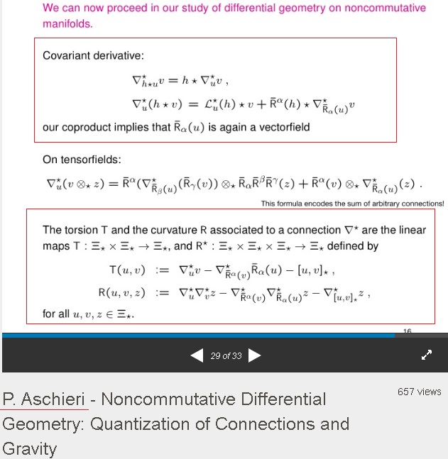
P. Aschieri’s Noncommutative Differential Geometry: Quantization of Connections and Gravity is an excellent read and a great backdrop to this post. Let me describe the non-Abelian Nambu-Goldstone model via the Lagrangian density:

${L^{NG}}\left( {A_\mu ^a} \right) = - \frac{1}{4}F_{\mu \nu }^a{F^{a\mu \nu }} - {J^{a\mu }}A_\mu ^a$

and the action-variation relative to ${B^a}$ , $A_{\bar \iota }^a$ gives us the EoMs:

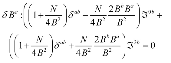
$\delta A_{\bar \iota }^a:\,{\Im ^{\bar \iota a}} + \frac{{{B^a}}}{{2{B^2}}}\left[ {{\Im ^{0b}} - {\Im ^{3b}}} \right]A_{\bar \iota }^a = 0$

with the following relations holding:

$\dot A_i^a = \frac{{\not \partial A_i^a}}{{\not \partial \Phi _B^b}}\dot \Phi _B^b \to \frac{{\not \partial \dot A_i^a}}{{\not \partial \dot \Phi _B^b}} = \frac{{\not \partial A_i^a}}{{\not \partial \Phi _B^b}}$

where the NANGM-action is given by:

$\int {{d^4}} x\prod _A^a\dot \Phi _A^a = \int {{d^4}} xE_i^a\dot A_i^a = \int {{d^4}} x\left( { - {E^{ai}}} \right)\dot A_i^a$

and:

$\dot \Phi _A^a = \frac{{\not \partial \Phi _A^a}}{{\not \partial A_i^b}}\dot A_i^b$

with conditions

$A_\mu ^a{A^{a\mu }} = {n^2}{M^2};\;{M^2} > 0;\,\mu = 0,1,2,3;\,a = 1,...,N$

${n_\mu }$

an oriented constant vector,

$M$

the Lorentz spontaneous symmetry breaking term,

${M^2} > 0;{\mkern 1mu} \quad \mu = 0,1,2,3;{\mkern 1mu} a = 1,...,N$

the Lorentz and gauge group indices with $N$ -generators.

It follows from

$A_\mu ^a{A^{a\mu }} = {n^2}{M^2}$

that there exists a nonzero vacuum expectation value:

$\left\langle {{A_\mu }} \right\rangle = {n_\mu }M$

guaranteeing the spontaneous symmetry breaking of Lorentz invariance and the existence of Goldstone bosons, which follows from Goldstone’s theorem. One then parametrizes the Non-Abelian Nambu-Goldstone Model via

$\left\{ {\begin{array}{*{20}{c}}{A_0^a = {B^a}\left( {1 + \frac{N}{{4{B^2}}}} \right)}\\{A_3^a = {B^a}\left( {1 - \frac{N}{{4{B^2}}}} \right)}\end{array}} \right.$

with:

$\left\{ {\begin{array}{*{20}{c}}{N = \left( {A_{\bar \iota }^bA_{\bar \iota }^b + {n^2}{M^2}} \right)}\\{4{B^2} \pm N \ne 0}\\{\bar \iota = 1,2}\end{array}} \right.$

After substituting

$A_0^a = {B^a}\left( {1 + \frac{N}{{4{B^2}}}} \right)$

in the Lagrangian density:

${L^{NG}}\left( {A_\mu ^a} \right) = - \frac{1}{4}F_{\mu \nu }^a{F^{a\mu \nu }} - {J^{a\mu }}A_\mu ^a$

we get the variation of the action relative to ${B^a}$ , $A_{\bar \iota }^a$ , yielding the equation of motion:

$\delta A_{\bar \iota }^a:\,{\Im ^{\bar \iota a}} + \frac{{{B^a}}}{{2{B^2}}}\left[ {{\Im ^{0b}} - {\Im ^{3b}}} \right]A_{\bar \iota }^a = 0$

with:

and

${\Im ^{\nu a}} \equiv {\left( {{{\not D}_\mu }{F^{\mu \nu }} - {J^\nu }} \right)^a}$

In the context of the SO(N) Yang Mills theory the equations of motion are ${\Im ^{0a}} = 0$

thus, we do not have current conservation:

${\not D_\nu }{J^{\nu a}} = 0$

due to the fact that the conditions:

$A_\mu ^a{A^{a\mu }} = {n^2}{M^2};\;{M^2} > 0;\,\mu = 0,1,2,3;\,a = 1,...,N$

are not gauge-invariant. However, by imposing the Gaussian condition:

${\Im ^{\bar \iota a}} = 0$

we recover gauge-invariance of the Yang Mills equations of motion. With invertible coordinate transformation:

$A_i^a = A_i^a\left( {\Phi _A^b} \right)$

its crucial transformation properties are:

and

$\dot \Phi _A^a = \frac{{\not \partial \Phi _A^a}}{{\not \partial A_i^b}}\dot A_i^b$

Let me proceed to the Hamiltonian aspect of the analytic-emergence relation between SU(N)-Gauge-Theory and the non-Abelian Nambu-Goldstone model

Getting the exact Hamiltonian, let its density be expressed in terms of the conjugated variables $\Phi _A^b$ , $\prod _A^b$ . Hence, given:

$A_0^a = A_0^a\left( {\Phi _A^b} \right)$

and the substitution in the Lagrangian density above, one can split:

${L^{NG}}\left( {A_\mu ^a} \right) = - \frac{1}{4}F_{\mu \nu }^a{F^{a\mu \nu }} - {J^{a\mu }}A_\mu ^a$

as such:

$\begin{array}{l}{L^{NG}}_{na}\left( {\Phi ,\dot \Phi } \right) = \frac{1}{2}E_i^aE_i^a - \\\frac{1}{2}B_i^aB_i^a - {J^{a\mu }}A_\mu ^a\end{array}$

with

$\left\{ {\begin{array}{*{20}{c}}{E_i^a = \dot A_i^a - {{\not D}_i}A_0^a}\\{B_i^a = \frac{1}{2}{\varepsilon _{ijk}}F_{jk}^a}\end{array}} \right.$

thus, we get the canonically conjugated momenta:

$\prod _A^a = \frac{{\not \partial {L^{NG}}_{na}\left( {\Phi ,\dot \Phi } \right)}}{{\not \partial \dot \Phi _A^a}} = E_i^b\frac{{\not \partial \dot A_i^b}}{{\not \partial \dot \Phi _A^a}} = E_i^b\frac{{\not \partial A_i^b}}{{\not \partial \Phi _A^a}}$

The inverse of

$A_i^a = A_i^a\left( {\Phi _A^b} \right)$

allows us to express $E_i^a$ as a function of the momenta $\prod _A^b$ of the Non-Abelian Nambu-Goldstone Model in the following form:

$E_i^b\left( {\Phi ,\prod } \right) = \frac{{\not \partial \,\Phi _A^a}}{{\not \partial A_i^b}}\prod _A^a$

Hence, and this is deep, the Wronskian of the system is

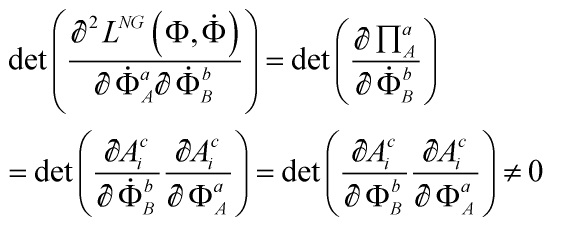
Which is gauge-invariant and exhibits parametric renormalization-group finiteness

Therefore, the Non-Abelian Nambu-Goldstone Model Hamiltonian density is:

$\begin{array}{l}{{\rm H}^d} = \prod _A^a\dot \Phi _A^a - \left( {\frac{1}{2}} \right.E_i^aE_i^a - \frac{1}{2}B_i^aB_i^a\\\left. { - {J^{a\mu }}A_\mu ^a} \right)\end{array}$

successively expressed as:

$\begin{array}{l}{{\rm H}^d}\left( {\Phi ,\prod } \right) = \frac{1}{2}E_i^aE_i^a + \frac{1}{2}B_i^aB_i^a\\ - \left( {{{\not D}_i}E_i^b - {J^{b0}}} \right)A_0^b + {J^{ai}}A_i^a\end{array}$

hence the dependence upon the canonical variables $\Phi$ , $\prod$ can be gotten via change of variables w.r.t.

$A_i^a = A_i^a\left( {\Phi _A^b} \right)$

$E_i^b\left( {\Phi ,\prod } \right) = \frac{{\not \partial \,\Phi _A^a}}{{\not \partial A_i^b}}\prod _A^a$

so the canonical variables satisfy the Poisson bracket algebra

$\left\{ {\Phi _A^a\left( x \right),\Phi _B^b\left( y \right)} \right\} = 0$

and

$\left\{ {\prod _A^a\left( x \right),\prod _B^b\left( y \right)} \right\} = 0$

and

$\left\{ {A_A^a\left( x \right),\prod _B^b\left( y \right)} \right\} = {\delta ^{ab}}{\delta _{AB}}{\delta ^3}\left( {x - y} \right)$

allowing us to derive the theory’s Hamiltonian action:

$\int {{d^4}} x\prod _A^a\dot \Phi _A^a = \int {{d^4}} xE_i^a\dot A_i^a = \int {{d^4}} x\left( { - {E^{ai}}} \right)\dot A_i^a$

with

$\left( { - {E^{ai}}} \right)$

the canonically conjugated momenta of $A_i^a$ , and so,

$\left( {\Phi ,\prod } \right) \to \left( {A,B} \right)$

hence, given:

$\begin{array}{l}{{\rm H}^d} = \prod _A^a\dot \Phi _A^a - \left( {\frac{1}{2}} \right.E_i^aE_i^a - \frac{1}{2}B_i^aB_i^a\\\left. { - {J^{a\mu }}A_\mu ^a} \right)\end{array}$

we get:

$A_0^a = \frac{{A_3^a}}{{\sqrt {A_3^bA_3^b} }}\left( {\sqrt {A_i^bA_i^b + {n^2}{M^2}} } \right)$

and since the transformations

$E_i^b\left( {\Phi ,\prod } \right) = \frac{{\not \partial \,\Phi _A^a}}{{\not \partial A_i^b}}\prod _A^a$

are generated from change-of-variables,

$A_0^a = A_0^a\left( {\Phi _A^b} \right)$

in coordinate space,

it follows from quantum-mechanics that the full transformation in the phase space is canonical. Thus, we can recover the Poisson bracket algebra

$\left\{ {\begin{array}{*{20}{c}}{\left\{ {A_i^a\left( x \right),A_j^b\left( y \right)} \right\} = 0}\\{\left\{ {{E^{ai}}\left( x \right),{E^{bj}}\left( y \right)} \right\} = 0}\\{\left\{ {A_i^a\left( x \right),{E^{bj}}\left( y \right)} \right\} = - {\delta ^{ab}}\delta _i^j{\delta ^3}\left( {x - y} \right)}\end{array}} \right.$

So, the time-evolution of the Gaussian functions under the dynamics of the NANGM is given by:

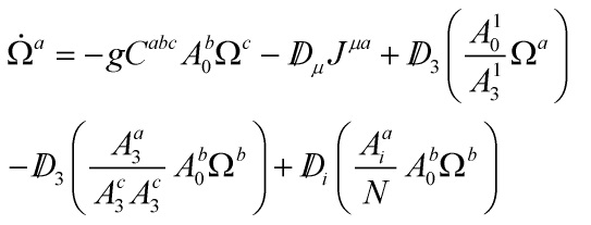
with $A_0^b$ determined by:

${L^{NG}}\left( {A_\mu ^a} \right) = - \frac{1}{4}F_{\mu \nu }^a{F^{a\mu \nu }} - {J^{a\mu }}A_\mu ^a$

When one imposes the Gaussian constraints as initial conditions:

$\left( {{\Omega ^a}\left( {t = {t_0}} \right) = 0} \right)$

the standard Yang-Mills equations of motion are validly recovered at $t = {t_0}$ , and given the antisymmetry of Maxwellian tensor, we get:

$0 = {\not D_\nu }{\Im ^{\nu a}} = {\not D_\nu }{\left( {{{\not D}_\mu }{F^{\mu \nu }} - {J^\nu }} \right)^a} = - {\not D_\nu }{J^{\nu a}} = 0$

at $t = {t_0}$ , and given

$\left\{ {\begin{array}{*{20}{c}}{{\Omega ^a}\left( {t = {t_0}} \right) = 0}\\{{{\not D}_\nu }{J^{\nu a}}\left| {_{t = {t_0}}} \right.}\end{array}} \right.$

one gets:

${\dot \Omega ^a}\left( {t = {t_0}} \right) = 0$

solving, we get:

$\begin{array}{l}{{\dot \Omega }^a}\left( {t = {t_0} + \delta {t_1}} \right) = {\Omega ^a}\left( {t = {t_0}} \right) + \\{{\dot \Omega }^a}\left( {t = {t_0}} \right)\delta {t_1} + ..., = 0\end{array}$

Therefore, the Yang Mills equations are now valid at $t = {t_0} + \delta {t_1}$ , entailing, by Maxwellian conditions, current conservation also at $t = {t_0} + \delta {t_1}$ .

So, we recover the SU(N) Yang-Mills theory by imposing the Gaussian laws as Hamiltonian metaplectic constraints, with functions ${N^a}$ adding $- {N^a}{\Omega ^a}$ to ${{\rm H}^d}$ , thus getting a redefinition:

$A_0^a + {N^a}: = {\Theta ^a}$

This leads to:

${{\rm H}^d} = \frac{1}{2}\left( {{{\tilde E}^2} + {{\tilde B}^2}} \right) - {\Theta ^a}{\Omega ^a} + J_i^a{A^{ia}}$

establishing, upon dimensional generalization, not only an emergent-relation between SU(N)-Gauge-Theory and Non-Abelian Nambu-Goldstone Model, but a stronger thesis: