Probing Multi-Field Inflation with Supersymmetric Quantum Mechanics

By George Shiber Saturday, February 11, 2017Friday, October 26, 2018 In Cosmology, Mathematical Physics, Mathematics, Philosophy Of Physics, Philosophy Of Science, Physics, Super String Theory, Supersymmetry, Witten Theory inflationary cosmology, Quantum Physics

Multi-scalar field cosmology is essential for solving the Wheeler-DeWitt equation in the context of quantum gravity. Here, I will test MFI with supersymmetric quantum mechanics based on Witten’s axiomatic approach. One can axiomatize multi-scalar field theory by the following conditions: 1) a Lagrangian containing up to second order derivatives of the fields, and 2) field equations that contain up to second order derivatives of the fields obeying:

with:

${{{\bar X}_{ij}} = \frac{1}{2}{\partial _a}{\pi _i}{\partial ^a}{\pi _j}}$

and $\frac{{\partial {A^{{i_1}...{i_m}}}}}{{\partial {X_{kl}}}}$ symmetric in all of its indices ${i_1}...{i_m},k,l$

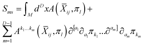
With the multi-field action in D dimensions having the form:

$S = \int {{d^D}} x\hat L\left( {{\pi _i},{\partial _a}{\pi _j},{\partial _b}{\partial _c}{\pi _k}} \right)$

whose Euler-Lagrange equations are given by:

$\frac{{\partial \hat L}}{{\partial {\pi _i}}} - {\partial _a}\left( {\frac{{\partial \hat L}}{{\partial {\pi _{ia}}}}} \right) + {\partial _a}{\partial _b}\left( {\frac{{\partial \hat L}}{{\partial {\pi _{iab}}}}} \right) = 0$

with a fourth derivatives constraint:

$\frac{{\partial \hat L}}{{\partial {\pi _{icd}}\partial {\pi _{iab}}}}{\pi _{i,abcd}}$

Thus, the universal multi-field action is:

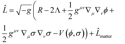
for the multi-fields $\left( {\sigma ,\phi } \right)$ , hence the corresponding field equations:

$\begin{array}{l}{G_{\alpha \beta }} + {g_{\alpha \beta }}\Lambda = + \frac{1}{2}\left( {{\nabla _\alpha }\phi {\nabla _\beta }\phi - \frac{1}{2}{g_{\alpha \beta }}{g^{\mu \nu }}{\nabla _\mu }\phi {\nabla _\nu }\phi } \right)\\ + \frac{1}{2}\left( {{\nabla _\alpha }\sigma {\nabla _\beta }\sigma - \frac{1}{2}{g_{\alpha \beta }}{g^{\mu \nu }}{\nabla _\mu }\sigma {\nabla _\nu }\sigma } \right)\\ - \frac{1}{2}{g_{\alpha \beta }}V\left( {\phi ,\sigma } \right) - 8\pi G{{\rm T}_{\alpha \beta }}\end{array}$

with:

$\begin{array}{c}{g^{\mu \nu }}{\phi _{,\mu \nu }} - {g^{\alpha \beta }}\Gamma _{\alpha \beta }^\nu {\nabla _\nu }\phi - \frac{{\partial V}}{{\partial \phi }} = 0\\ \Leftrightarrow \\{{\hat \bigcirc }_L}\phi - \frac{{\partial V}}{{\partial \phi }} = 0\end{array}$

$\begin{array}{c}{g^{\mu \nu }}{\sigma _{,\mu \nu }} - {g^{\alpha \beta }}\Gamma _{\alpha \beta }^\nu {\nabla _\nu }\sigma - \frac{{\partial V}}{{\partial \sigma }} = 0\\ \Leftrightarrow \\{{\hat \bigcirc }_L}\sigma - \frac{{\partial V}}{{\partial \sigma }} = 0\end{array}$

with:

${\rm T}_{;\mu }^{\mu \nu } = 0\,\;;\,\;{\rm T} = {\rm{P}}{g_{\mu \nu }} + \left( {{\rm{P}} + \rho } \right){\tilde w_\mu }{\tilde w_\nu }$

$\rho$ the energy density, ${\rm{P}}$ the pressure, and ${\tilde w_\mu }$ the velocity, satisfying ${\tilde w_\mu }{\tilde w^\mu } = - 1$ .

The multi-scalar field cosmological paradigm requires the two canonical fields $\left( {\sigma ,\phi } \right)$ , the action of a universe based on such fields, the cosmological term contribution, and matter as a perfect fluid content, and is given by:

Our metric has the form:

${\rm{d}}{{\rm{s}}^2} = - {\rm{N}}\left( t \right){\rm{d}}{{\rm{t}}^2} + {e^{2\Omega \left( {\rm{t}} \right)}}{\left( {{e^{2\beta \left( {\rm{t}} \right)}}} \right)_{{\rm{ij}}}}{\omega ^{\rm{i}}}{\omega ^{\rm{j}}}$

with ${\beta _{{\rm{ij}}}}\left( {\rm{t}} \right)$ a 3 x 3 diagonal matrix,

${\beta _{{\rm{ij}}}} = {\rm{diag}}\left( {{\beta _ + } + \sqrt 3 {\beta _ - },{\beta _ + } - \sqrt 3 {\beta _ - }, - 2{\beta _ + }} \right)$

and $\Omega \left( t \right)$ is a scalar and ${\omega ^{\rm{i}}}$ are one-forms that characterize each cosmological Bianchi type model, and obey the form:

${\rm{d}}{\omega ^{\rm{i}}} = \frac{1}{2}C_{{\rm{jk}}}^{\rm{i}}{\omega ^{\rm{j}}} \wedge {\omega ^{\rm{k}}}$

and $C_{{\rm{jk}}}^{\rm{i}}$ are structure constants of the corresponding model. Hence, in Misner’s parametrization, we get:

$\begin{array}{l}{\rm{ds}}_{\rm{I}}^2 = - {{\rm{N}}^2}{\rm{d}}{{\rm{t}}^2} + {e^{2\Omega + 2{\beta _ + } + 2\sqrt 3 \beta }} - {\rm{d}}{{\rm{x}}^2}\\ + \,{e^{2\Omega + 2{\beta _ + } - 2\sqrt 3 \beta }} - {\rm{d}}{{\rm{y}}^2} + {e^{2\Omega - 4{\beta _ + }}}{\rm{d}}{{\rm{z}}^2}\end{array}$

with the anisotropic conditions:

$\left\{ {\begin{array}{*{20}{c}}{{{\rm{R}}_{\rm{1}}} = {e^{\Omega + {\beta _ + } + \sqrt 3 {\beta _ - }}}}\\{{{\rm{R}}_{\rm{2}}} = {e^{\Omega + {\beta _ + } - \sqrt 3 {\beta _ - }}}}\\{{{\rm{R}}_{\rm{3}}} = {e^{\Omega - 2{\beta _ + }}}}\end{array}} \right.$

So the lagrangian density above can be written as:

$\begin{array}{l}{{\hat L}_{\rm{I}}} = {e^{3\Omega }}\left[ {6\frac{{{{\dot \Omega }^2}}}{{\rm{N}}} - 6\frac{{\dot \beta _ - ^2}}{{\rm{N}}} - 6\frac{{\dot \beta _ - ^2}}{{\rm{N}}} - 6\frac{{{{\dot \varphi }^2}}}{{\rm{N}}} - 6\frac{{{{\dot \varsigma }^2}}}{{\rm{N}}}} \right.\\ + {\rm{N}}\left. {\left( {V\left( {\varphi ,\varsigma } \right) + 2\Lambda + 16\pi G\rho } \right)} \right]\end{array}$

with overdot denotes time derivative, with the re-scaling:

$\left\{ {\begin{array}{*{20}{c}}{\phi = \sqrt {12} \varphi }\\{\sigma \sqrt {12} \varsigma }\end{array}} \right.$

And the momenta are defined as:

$\left\{ {\begin{array}{*{20}{c}}{\prod\nolimits_{{q^i}} = \frac{{\partial \hat L}}{{\partial {q^i}}}}\\{{q^i} = \left( {{\beta _ \pm },\Omega ,\varphi ,\varsigma } \right)}\end{array}} \right.$

and:

$\left\{ {\begin{array}{*{20}{c}}{{\Pi _\Omega } = \frac{{\partial \hat L}}{{\partial \dot \Omega }} = \frac{{12{e^{3\Omega }}\dot \Omega }}{{\rm{N}}}}\\{ \to \dot \Omega = \frac{{{\rm{N}}{\Pi _\Omega }}}{{12}}{e^{ - 3\Omega }}}\end{array}} \right.$

$\left\{ {\begin{array}{*{20}{c}}{{\Pi _ \pm } = \frac{{\partial \hat L}}{{\partial {{\dot \beta }_ \pm }}} = \frac{{12{e^{3\Omega }}{{\dot \beta }_ \pm }}}{{\rm{N}}}}\\{ \to {{\dot \beta }_ \pm } = - \frac{{{\rm{N}}{\Pi _ \pm }}}{{12}}{e^{ - 3\Omega }}}\end{array}} \right.$

$\left\{ {\begin{array}{*{20}{c}}{{\Pi _\varphi } = \frac{{\partial \hat L}}{{\partial \dot \varphi }} = \frac{{12{e^{3\Omega }}\dot \varphi }}{{\rm{N}}}}\\{ \to \dot \varphi = - \frac{{{\rm{N}}{\Pi _\varphi }}}{{12}}{e^{ - 3\Omega }}}\end{array}} \right.$

$\left\{ {\begin{array}{*{20}{c}}{{\Pi _\varsigma } = \frac{{\partial \hat L}}{{\partial \dot \varsigma }} = \frac{{12{e^{3\Omega }}\dot \varsigma }}{{\rm{N}}}}\\{ \to \dot \varsigma = - \frac{{{\rm{N}}{\Pi _\varsigma }}}{{12}}{e^{ - 3\Omega }}}\end{array}} \right.$

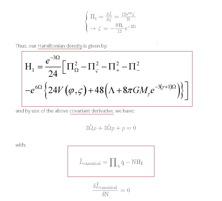
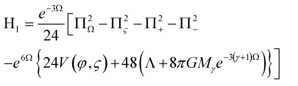
Thus, our Hamiltonian density is given by:

and by use of the above covariant derivative, we have:

$3\dot \Omega \rho + 3\dot \Omega p + p = 0$

with:

${\hat L_{{\rm{canonical}}}} = \prod\nolimits_{\rm{q}} {{\rm{\dot q}}} - {\rm{N}}{{\rm H}_{\rm{I}}}$

$\frac{{\delta {{\hat L}_{{\rm{canonical}}}}}}{{\delta {\rm{N}}}} = 0$

and:

${{\rm H}_{\rm{I}}} = 0$

and the density solution:

$\rho = {{\rm{M}}_\gamma }{e^{ - 3\left( {1 + \gamma } \right)\,\Omega }}$

The Wheeler-DeWitt equation

Hence, our first approximation of the Wheeler-DeWitt equation is:

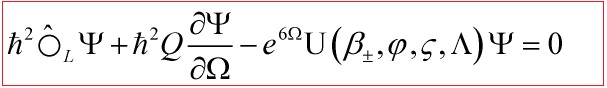
with:

${\hat \bigcirc _L} = - \frac{{{\partial ^2}}}{{\partial {\Omega ^2}}} + \frac{{{\partial ^2}}}{{\partial {\varsigma ^2}}} + \frac{{{\partial ^2}}}{{\partial {\varphi ^2}}} + \frac{{{\partial ^2}}}{{\partial \beta _ - ^2}} + \frac{{{\partial ^2}}}{{\partial \beta _ + ^2}}$

the d’Alambertian in the coordinates:

${q^\mu } = \left( {\Omega ,{\beta _ \pm },\varsigma ,\varphi } \right)$

with the ${\rm{U}}$ potential that couples to the wave-function $\psi$ and gives the whole quantum dynamics by the following equation:

${\rm H}\psi = \left( {{g^{\mu \nu }}{\nabla _\mu }{\nabla _\nu } - V\left( {{q^\mu }} \right)} \right)\psi = 0$

with:

$\psi = {\rm{R}}\left( {{q^\mu }} \right){e^{\frac{i}{\hbar }S\left( {{q^\mu }} \right)}}$

Using the following ansatz for the wavefunction:

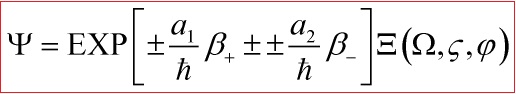
Hence, our Wheeler–DeWitt equation equation is:

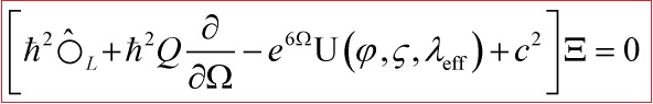
with:

$\left\{ {\begin{array}{*{20}{c}}{{c^2} = \left( {a_1^2 + a_2^2} \right)}\\{{{\hat \bigcirc }_L} = {\ell ^\mu }\left( {\Omega ,\varsigma ,\varphi } \right)}\end{array}} \right.$

and:

$\Xi \left( {{\ell ^\mu }} \right) = {\rm{W}}\left( {{\ell ^\mu }} \right){e^{ - \frac{{{S_\hbar }}}{\hbar }\left( {{\ell ^\mu }} \right)}}$

where ${S_\hbar }\left( {{\ell ^2}} \right)$ is the superpotential function, and ${\rm{W}}$ is the probability amplitude.

Let us now utilize the mathematics of supersymmetric quantum mechanics to probe the Wheeler–DeWitt equation and the superpotential via Witten’s formalism of finding the supersymmetric supercharges operators $Q$ and $\bar Q$ that produce a super-Hamiltonian ${{\rm{H}}_{{\rm{ss}}}}$ , where the Wheeler–DeWitt equation can be derived as the bosonic sector of this super-Hamiltonian in the superspace. The right method to supersymmetrize a bosonic Lagrangian is to consider the true supersymmetry transformation in the superfield scheme into the bosonic Lagrangian, then the fermionic terms will emerge in a natural way.

In this Witten-method, our supercharges for the 3-D case are:

$Q = {\psi ^\mu }\left[ { - \hbar {\partial _{{{\rm{q}}^\mu }}} + \frac{{\partial S}}{{\partial {{\rm{q}}^\mu }}}} \right]$

$\bar Q = {\bar \psi ^\nu }\left[ { - \hbar {\partial _{{{\rm{q}}^\nu }}} + \frac{{\partial S}}{{\partial {{\rm{q}}^\nu }}}} \right]$

where $S$ is defined implicitly by the following equation:

$S = \frac{{{e^{3\Omega }}}}{\mu }g\left( \varphi \right){\rm{h}}\left( \varsigma \right)$

and the super-algebra for the variables $\left( {{\psi ^\mu },{{\bar \psi }^\nu }} \right)$ is given by:

$\left\{ {\begin{array}{*{20}{c}}{\left\{ {{\psi ^\mu },{{\bar \psi }^\nu }} \right\} = {\eta ^{\mu \nu }}}\\{\left\{ {{\psi ^\mu },{\psi ^\nu }} \right\} = 0}\\{\left\{ {{{\bar \psi }^\mu },{{\bar \psi }^\nu }} \right\} = 0}\end{array}} \right.$

Under the representation:

${\psi ^\nu } = {\theta ^\nu }{\rm{y}}{\bar \psi ^\mu } = {\eta ^{\mu \nu }}\frac{\partial }{{\partial {\theta ^\nu }}}$

the superspace Hamiltonian takes the form:

${{\rm{H}}_{{\rm{ss}}}} = \left\{ {Q,\bar Q} \right\} = {H_0} + \hbar \frac{{{\partial ^2}S}}{{\partial {{\rm{q}}^\mu }\partial {{\rm{q}}^\nu }}}\left[ {{\psi ^\mu },{{\bar \psi }^\nu }} \right]$

with:

${H_0} = {\hat \bigcirc _L} - {\rm{U}}\left( {{{\rm{q}}^\mu }} \right)$

being the standard Wheeler–DeWitt equation, ${\hat \bigcirc _L}$ the 3-D d’Alambertian in the ${{\rm{q}}^\mu }$ coordinates with ${\eta _{\mu \nu }} = {\rm{diag}}\left( { - 1,1,1} \right)$ , and $\left\{ {\,,\,} \right\}$ and $\left[ {\,,\,} \right]$ represent the anticommutator and the commutator respectively. The supercharges and the super-Hamiltonian satisfy the following algebra:

$\left\{ {\begin{array}{*{20}{c}}{\left\{ {Q,\bar Q} \right\} = {{\rm{H}}_{{\rm{ss}}}}}\\{\left[ {{{\rm{H}}_{{\rm{ss}}}},Q} \right] = \left[ {{{\rm{H}}_{{\rm{ss}}}},\bar Q} \right] = 0}\end{array}} \right.$

Hence, our supersymmetric physical states are selected by the constraints:

$\left\{ {\begin{array}{*{20}{c}}{Q\Psi = 0}\\{\bar Q\Psi = 0}\end{array}} \right.$

which reduces the problem of finding supersymmetric ground states because the energy is known a priori and the factorization of:

${{\rm{H}}_{{\rm{ss}}}}\left| \Psi \right\rangle = 0$

into

$\left\{ {\begin{array}{*{20}{c}}{Q\Psi = 0}\\{\bar Q\Psi = 0}\end{array}} \right.$

yields a first-order equation for the ground state wave-function due to the sovability of the bosonic Hamiltonians and normalization just means that supersymmetry is quantum mechanically unbroken.

In the 3-D Grassmannian variable-representation, the wave-function has the following decomposition:

$\begin{array}{c}\Psi = {{\tilde A}_ + } + {{\tilde B}_\nu }{\theta ^\mu } + \frac{1}{2}{\varepsilon _{\mu \nu \lambda }}{C^\lambda }{\theta ^\mu }{\theta ^\nu }\\ + {{\tilde A}_ - }{\theta ^0}{\theta ^1}{\theta ^2}\end{array}$

and with the ansatz:

${\tilde B_\nu } = \frac{{\partial {{\rm{f}}_ + }\left( {{{\rm{q}}^\nu }} \right)}}{{\partial {{\rm{q}}^\nu }}}{e^{\frac{{{S_{\left( {\rm{q}} \right)}}}}{\hbar }}}$

introduced into

$\left\{ {\begin{array}{*{20}{c}}{Q\Psi = 0}\\{\bar Q\Psi = 0}\end{array}} \right.$

and

where $S$ is the superpotential function obtained as a solution for the Einstein-Hamilton-Jacobi equation, the following identity:

${\left( {\nabla {S_\hbar }} \right)^2} - \tilde U = 0$

yields the master equation for the auxiliary function ${{\rm{f}}_ + }$ :

$\hbar {\hat \bigcirc _L}{{\rm{f}}_ + } + 2{\eta ^{\mu \nu }}\frac{{\partial S}}{{\partial {{\rm{q}}^\mu }}}\frac{{\partial {{\rm{f}}_ + }}}{{\partial {{\rm{q}}^\nu }}} = 0$

with:

$\frac{1}{2}{\varepsilon _{\mu \nu \lambda }}{C^\lambda }{\theta ^\alpha }{\theta ^\mu }{\theta ^\nu } = {C^\alpha }{\theta ^0}{\theta ^1}{\theta ^2}$

and with the following ansatz:

${C^\mu } = {\eta ^{\mu \nu }}\frac{{\partial {{\rm{f}}_ - }}}{{\partial {{\rm{q}}^\nu }}}{e^{ - \frac{{{S_{\left( {\rm{q}} \right)}}}}{\hbar }}}$

we get the second master equation in the form:

$\hbar {\hat \bigcirc _L}{{\rm{f}}_ - } - 2{\eta ^{\mu \nu }}\frac{{\partial S}}{{\partial {{\rm{q}}^\mu }}}\frac{{\partial {{\rm{f}}_ - }}}{{\partial {{\rm{q}}^\nu }}} = 0$

allowing us to get the reduction to:

$\hbar {\hat \bigcirc _L}{{\rm{f}}_ \pm } \pm 2{\eta ^{\mu \nu }}\frac{{\partial S}}{{\partial {{\rm{q}}^\mu }}}\frac{{\partial {{\rm{f}}_ \pm }}}{{\partial {{\rm{q}}^\nu }}} = 0$

and the equations for the functions ${\tilde A_ \pm }$ are:

$\left[ {\hbar \frac{\partial }{{\partial {{\rm{q}}^\mu }}} \pm \frac{{\partial S}}{{\partial {{\rm{q}}^\mu }}}} \right]{\tilde A_ \pm } = 0$

with solutions:

${\tilde A_ \pm } = {a_{0 \pm }}{e^{ \pm \frac{1}{\hbar }S}}$

with ${a_{0 \pm }}$ the integration constants.

To solve our equation:

$\hbar {\hat \bigcirc _L}{{\rm{f}}_ \pm } \pm 2{\eta ^{\mu \nu }}\frac{{\partial S}}{{\partial {{\rm{q}}^\mu }}}\frac{{\partial {{\rm{f}}_ \pm }}}{{\partial {{\rm{q}}^\nu }}} = 0$

we need to write it as a homogeneous linear equation of second degree:

${\hat \bigcirc _L}{{\rm{W}}_ \pm } = {{\rm{W}}_ \pm }g\left( {{{\rm{q}}^\mu }} \right)$

and we do this by introducing into it the ansatz:

${{\rm{f}}_ \pm } = {{\rm{W}}_ \pm }\left( {{{\rm{q}}^\mu }} \right){e^{ \pm \phi \left( {{{\rm{q}}^\mu }} \right)/\hbar }}$

This way, we obtain a wave-like equation:

${\hat \bigcirc _L}{{\rm{W}}_ \pm } \pm {{\rm{W}}_ \pm }{\hat \bigcirc _L}S - {{\rm{W}}_ \pm }{\left( {\nabla S} \right)^2} = 0$

with:

$g\left( {{{\rm{q}}^\mu }} \right) = \left( {\nabla S} \right) \mp {\hat \bigcirc _L}S$

and:

${\hat \bigcirc _L}{{\rm{W}}_ \pm } = g\left( {{{\rm{q}}^\mu }} \right){{\rm{W}}_ \pm }$

The following wave-like ansatz:

${{\rm{W}}_ \pm } = {\beta _ \pm }{e^{ \mp * }}$

suffices to solve, yielding a condition on the ${\rm{s}}$ function:

$\left[ {{{\left( {\nabla {\rm{s}}} \right)}^2} \mp \,{{\hat \bigcirc }_L}{\rm{s}}} \right] = \left[ {{{\left( {\nabla {\rm{S}}} \right)}^2} \mp \,{{\hat \bigcirc }_L}{\rm{S}}} \right]$

where the following conditions hold:

$\left\{ {\begin{array}{*{20}{c}}{{\rm{s}} = S \mp {\rm{h}}\left( {{{\rm{q}}^\mu }} \right)}\\{{\rm{h}}\left( {{{\rm{q}}^\mu }} \right) \equiv {{\rm{m}}_\mu }{{\rm{q}}^\mu }}\end{array}} \right.$

Allowing us to construct the following term:

$\left[ {{{\left( {\nabla {\rm{s}}} \right)}^2} \mp \,{{\hat \bigcirc }_L}{\rm{s}}} \right]$

satisfying:

$\begin{array}{l}{\left( {\nabla {\rm{s}}} \right)^2} \mp {{\hat \bigcirc }_L}{\rm{s}}{\left( {\nabla {\rm{S}}} \right)^2} \mp \,{{\hat \bigcirc }_L}S \pm \\2{\eta ^{\mu \alpha }}{{\rm{m}}_\alpha }\frac{{\partial S}}{{\partial {{\rm{q}}^\mu }}} + {{\rm{m}}^\mu }{{\rm{m}}_\mu }\end{array}$

Now, for:

$2{{\rm{m}}^\mu }\frac{{\partial S}}{{\partial {{\rm{q}}^\mu }}} \mp {{\rm{m}}^\mu }{{\rm{m}}_\mu } = 0$

we must consider the two cases, one with taking the constant $c$ into account and one without.

For $c \ne 0$ and with our superpotential. In this situation,

$2{{\rm{m}}^\mu }\frac{{\partial S}}{{\partial {{\rm{q}}^\mu }}} \mp {{\rm{m}}^\mu }{{\rm{m}}_\mu } = 0$

gives the following equation:

$\begin{array}{l}\frac{{{e^{3\Omega }}g{\rm{h}}}}{\mu }\left[ { - 6{{\rm{m}}_0} + 6{{\rm{m}}_1}\frac{{{\eta _1}}}{{{{\rm{b}}_3}}}} \right] - \\2c\left( { - {{\rm{m}}_0}{{\rm{b}}_1} + {{\rm{m}}_1}{{\rm{b}}_2} + {{\rm{m}}_2}{{\rm{b}}_3}} \right) + {\rm{m}}_0^2 - {\rm{m}}_1^2 - {\rm{m}}{2^2} = 0\end{array}$

with vector solutions:

$\left\{ {\begin{array}{*{20}{c}}{{{\rm{m}}_\mu } = \left( {2c{{\rm{b}}_1},2c{{\rm{b}}_2},2c{{\rm{b}}_3}} \right)}\\{{{\rm{b}}_1} \equiv {\eta _1} + {\eta _2}}\end{array}} \right.$

For $c = 0$ and with our superpotential. In this situation, we need to separate the following two independent equations:

$\left\{ {\begin{array}{*{20}{c}}{{{\rm{m}}^\mu }{{\rm{m}}_\mu } = 0}\\{{\eta ^{\mu \alpha }}{{\rm{m}}_\alpha }\frac{{\partial S}}{{\partial {{\rm{q}}^\mu }}} = 0}\end{array}} \right.$

where:

${{\rm{m}}^\mu }{{\rm{m}}_\mu } = 0$

entails that ${{\rm{m}}_\mu }$ is a vector of null measure, and:

${\eta ^{\mu \alpha }}{{\rm{m}}_\alpha }\frac{{\partial S}}{{\partial {{\rm{q}}^\mu }}} = 0$

entails:

$\frac{{\partial S}}{{\partial \Omega }}{{\rm{m}}_0} = \frac{{\partial S}}{{\partial \phi }}{{\rm{m}}_1} + \frac{{\partial S}}{{\partial \sigma }}{{\rm{m}}_2}$

Now, when we use the superpotential function:

$S = \frac{{{e^{3\Omega }}}}{\mu }g\left( \varphi \right){\rm{h}}\left( \varsigma \right)$

we get the following structural relations:

$\left\{ {\begin{array}{*{20}{c}}{{\rm{g}}\left( \phi \right) = {g_0}{e^{{\varepsilon _1}\Delta \phi }}}\\{{\rm{h}}\left( \sigma \right) = {{\rm{h}}_0}{g_0}{e^{{\varepsilon _2}\Delta \phi }}}\end{array}} \right.$

for $\left( {g\left( \varphi \right){\rm{;h}}\left( \varsigma \right)} \right)$ , where the constants are:

$\left\{ {\begin{array}{*{20}{c}}{{\varepsilon _1} = \frac{{3{{\rm{m}}_0}{{\rm{n}}_1}}}{{{{\rm{m}}_2}}}}\\{{\varepsilon _2} = \frac{{3{{\rm{m}}_0}{{\rm{n}}_2}}}{{{{\rm{m}}_1}}}}\end{array}} \right.$

Hence, supersymmetric quantum mechanics puts the exact constraints on the family of potential fields corresponding to the inflaton exponential Hubble-Fredholm integral.

In the scenario where both equations have no null solution, the solution for the function ${{\rm{f}}_ \pm }$ has the following structure:

${{\rm{f}}_ \pm } = {{\rm{b}}_ \pm }{e^{{{\rm{m}}_\alpha }{{\rm{q}}^\alpha }}}$

thus ${\tilde B_\mu }$ and ${C^\mu }$ reduce to:

${\tilde B_\mu } = {{\rm{b}}_ + }{{\rm{m}}_\mu }{e^{{{\rm{m}}_\mu }{{\rm{q}}^\mu }}}{e^{\frac{S}{\hbar }}}$

${C^\mu } = {\eta ^{\mu \nu }}{{\rm{b}}_ - }{{\rm{m}}_\nu }{e^{{{\rm{m}}_\alpha }{{\rm{q}}^\alpha }}}{e^{ - \frac{S}{\hbar }}}$

Our method above was used to obtain supersymmetric quantum solutions for all cosmological bianchi class A models in Sáez-Ballester theory.

From our superpotential function above, it follows that the only form for $S$ in which our equations are fulfilled, is when the functions ${\rm{g}}$ and ${\rm{h}}$ have exponential behavior. So in a supersymmetric way, the calculation by means of the Grassmannian variables of ${\left| \Psi \right|^2}$ given by:

is:

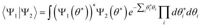
where $*$ is implicitly defined by:

${\left( {C{\theta _1}...{\theta _n}} \right)^ * } = \theta _n^ * ...\theta _1^ * {C^ * }$

with the standard algebra for the Grassmannian numbers ${\theta _i}{\theta _j} = - {\theta _j}{\theta _i}$ . The integration rules over these numbers are given by:

$\int {{\theta _1}\theta _1^ * ...{\theta _n}\theta _n^ * d\theta _n^ * d{\theta _n}...d\theta _1^ * d{\theta _1} = 1}$

with:

$\int {d\theta _i^ * } = \int {d{\theta _i}} = 0$

and we get:

${\Psi _1} = {\Psi _2} = \Psi$

Thus, Grassmannian integration yields:

$\begin{array}{l}{\left| \Psi \right|^2} = {{\tilde A}_ + }{A_ + } + {{\tilde A}_ - }{A_ - } + {{\tilde B}_0}{B_0} + \\{{\tilde B}_1}{B_1} + {{\tilde B}_2}{B_2} + {{\tilde C}^0}{C^0} + {{\tilde C}^1}{C^1} + {{\tilde C}^2}{C^2}\end{array}$

thus supersymmetric quantum mechanics yields the required probability density:

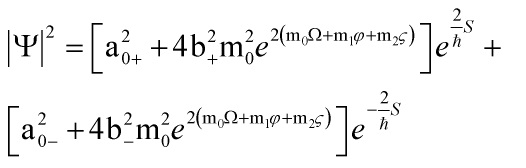
giving us a supersymmetric quantum canonical quantization of the multi-scalar field cosmology of the anisotropic Bianchi type I model and the exact supersymmetric quantum solutions to the Wheeler-DeWitt equation are derived under the ansatz to the wave function:

$\Psi \left( {{\ell ^\mu }} \right) = {e^{\frac{{{{\rm{a}}_1}}}{\hbar }{\beta _ + } + {\rm{i}}\frac{{{{\rm{a}}_1}}}{\hbar }{\beta _ - }}}{\rm{W}}\left( {{\ell ^\mu }} \right){e^{ - \frac{{S\left( {{\ell ^\mu }} \right)}}{\hbar }}}$