Quantum Geometry and Nonlinear Phase Spaces

By George Shiber Wednesday, February 1, 2017Saturday, August 17, 2019 In Mathematical Physics, Mathematics, Physics, Super String Theory Hamiltonian analysis, Nonlinear Phase Spaces

It was Born who argued, correctly, that the geometric structure of quantized spacetime should reflect the same structure of the corresponding momentum space and that the phase space of values of a given quantum field is isomorphic to a nontrivial metaplectic manifold. This is true of string-theory, as the Tseytlin formulation entails. Recall, with $M$ a symplectic structure:

${B^s} = \frac{1}{2}{B^s}_{ab}d{y^a} \wedge d{y^b}$

one quantizes spacetime via its quantum-phase Poisson algebraic structure:

${\theta ^{ab}} \equiv {\left( {{B^{ - 1}}} \right)^{ab}}$

Hence, we have, for: $f,g \in {\mathbb{C}^\infty }\left( M \right)$ , the following:

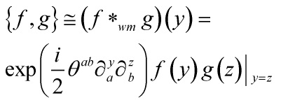
Thus, the noncommutative algebra of operators is isomorphic to the deformed algebra of functions defined by the Weyl-Moyal product:

We then define a noncommutative space ${\mathbb{R}^{2n}}$ via the commutation relation:

${\left[ {{y^a},{y^b}} \right]_{{ * _{wm}}}} = i{\theta ^{ab}}$

that allows us to interpret it as a noncommutative phase-space with Poisson structure given by ${\theta ^{ab}}$ .

Now, any field $\hat \phi \in {{\rm A}_\theta }$ can be expanded in terms of the complete-operator-basis:

$\left\{ {\begin{array}{*{20}{c}}{{{\rm A}_\theta } = \left\{ {\left| m \right\rangle \left\langle n \right|,n,m = 0,...} \right\}}\\{\hat \phi \left( {x,y} \right)\sum\limits_{n,m} {{M_{mn}}\left| m \right\rangle \left\langle n \right|} }\end{array}} \right.$

with ${{\rm A}_\theta }$ a C*-algebra, that is:

${e^{ik \cdot y}}{ * _{wm}}f\left( y \right){ * _{wm}}{e^{ - ik \cdot y}} = f\left( {y + \theta \cdot k} \right)$

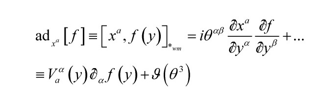
in infinitesimal form:

${\left[ {{y^a},f} \right]_{{ * _{wm}}}} = i{\theta ^{ab}}{\not \partial _b}f$

The coordinates ${y^a}$ in a gauge-theoretic setting will get promoted to the covariant coordinates defined by:

${x^a}\left( y \right) \equiv {y^a} + {\theta ^{ab}}{\hat A_b}\left( y \right)$

and thus:

${\left[ {{y^a},f} \right]_{{ * _{wm}}}} = i{\theta ^{ab}}{\not \partial _b}f$

get covariantized as:

and from

${\theta ^{ab}} \equiv {\left( {{B^{ - 1}}} \right)^{ab}}$

we get a quantum-geometry relation:

${V_a}\left( y \right) \equiv V_a^\alpha \left( y \right){\not \partial _\alpha }$

constituting an orthonormal frame and defining vielbeins of a gravitational metric.

Since Darboux’s theorem in symplectic geometry is equivalent to the equivalence-principle in general relativity, it follows that the induced D-manifold defined by the metaplectic generalized quantum geometry continuously interpolates between a symplectic geometry $\left( {\left| {\kappa {B^s}{g^{ - 1}}} \right| \gg 1} \right)$ and a Riemannian geometry $\left( {\left| {\kappa {B^s}{g^{ - 1}}} \right| \ll 1} \right)$ .

To justify Born’s thesis, let us simplify and work on a 4-D manifold ${\mathbb{R}^{3,1}}$ and without loss of generality, a scalar field defined on it. The Hamiltonian in the Fourier representation is:

$H = \frac{1}{2}\sum\limits_{\rm{k}} {\left( {\pi _{\rm{k}}^2 + {k^2}\phi _{\rm{k}}^2} \right)}$

with $k \equiv \sqrt {{\rm{k}} \cdot {\rm{k}}}$ , and the phase-space for each mode ${\rm{k}}$ is:

${\Gamma _{\rm{k}}}: = {T^ * }\left( \mathbb{R} \right) = \left( {{\phi _{\rm{k}}},{\pi _{\rm{k}}}} \right) \in {\mathbb{R}^2}$

with Poisson bracket $\left( {{\phi _{\rm{k}}},{\pi _{\rm{k}}}} \right) = 1$ and total field phase-space $\Gamma = \prod\nolimits_{\rm{k}} {{\Gamma _{\rm{k}}}}$ and with no loss of content, we can take: ${\Gamma _{\rm{k}}} = {S^2},\;\forall {\rm{k;}}\;\quad {S^2}\;{\rm{a}}\;{\rm{sphere}}$ . Our symplectic form is given by the area form

$\omega = J\sin \theta d\varphi \wedge d\theta$

locally:

$\omega = \sum\limits_{i = 1}^n {{\rm{d}}{x^{n + i}}} \wedge {\rm{d}}{x^i}$

and the Hamiltonian vector field ${X_f}$ associated to a smooth function $f$ can be locally written as:

${X_f} = \sum\limits_{i = 1}^n {\frac{{\partial f}}{{\partial {x^{n + i}}}}} \frac{\partial }{{\partial {x^i}}} - \frac{{\partial f}}{{\partial {x^i}}}\frac{\partial }{{\partial {x^{n + i}}}}$

and for any smooth curve $\varphi$ , the Hamilton-equation for the Hamiltonian $f$ is:

$\frac{{{\rm{d}}\varphi \left( t \right)}}{{{\rm{d}}t}} = {X_f}\left( {\varphi \left( t \right)} \right)$

Standard definition: with $\Phi :N \to N$ a diffeomorphism of a smooth manifold $N$ onto itself, the canonical lift of $\Phi$ to the cotangent bundle is the transpose of the vector bundles isomorphism

$T\left( {{\Phi ^{ - 1}}} \right) = {\left( {T\Phi } \right)^{ - 1}}:TN \to TN$

So, letting $\hat \Phi$ be the canonical lift of $\Phi$ to the cotangent bundle, we have for all $x \in N,\,\;\xi \in T_x^ * N,\;\nu \in {T_{\Phi \left( x \right)}}N$ :

$\left\langle {\hat \Phi \left( \xi \right),\nu } \right\rangle = \left\langle {\xi ,{{\left( {T\Phi } \right)}^{ - 1}}\left( \nu \right)} \right\rangle$

thus allowing us to derive:

$\int_{{S^2}} \omega = 4\pi J$

and $J$ being the non-linearity scale and the covering angular coordinates being: $\varphi$ and $\theta$ . The field variables $\left( {{\phi _{\rm{k}}},{\pi _{\rm{k}}}} \right)$ are parametrizable in terms of $\varphi$ and $\theta$ as such:

$\left\{ {\begin{array}{*{20}{c}}{{R^{ - 1}}{\phi _{\rm{k}}} = \varphi - \pi \in \left[ { - \pi ,\pi } \right)}\\{R{J^{ - 1}}{\pi _{\rm{k}}} = \frac{\pi }{2} - \theta \in \left[ { - \frac{\pi }{2},\frac{\pi }{2}} \right]}\end{array}} \right.$

with a dimensional constant. Our symplectic form reduces to:

$\omega = \cos \left( {\frac{R}{J}{\pi _{\rm{k}}}} \right)d{\pi _{\rm{k}}} \wedge d{\phi _{\rm{k}}}$

with corresponding Poisson bracket:

$\left\{ {{\phi _{\rm{k}}},{\pi _{\rm{k}}}} \right\} = \sec \left( {R{J^{ - 1}}{\pi _{\rm{k}}}} \right)$

and the spin-coordinates are:

$\left\{ {\begin{array}{*{20}{c}}{{J_{\left( x \right)}}: = J\sin \theta \cos \varphi }\\{{J_{\left( y \right)}}: = J\sin \theta \sin \varphi }\\{{J_{\left( z \right)}}J\cos \theta }\end{array}} \right.$

satisfying:

$J_{\left( x \right)}^2 + J_{\left( y \right)}^2 + J_{\left( z \right)}^2 = {J^2}$

with the ${J_i}$ ‘s spanning the corresponding $S{U_L}\left( 2 \right)$ Lie algebra:

$\left\{ {{J_i},{J_j}} \right\} = {\varepsilon _{ijk}}{J^k}$

To derive a Hamiltonian that is globally well-defined, has the minimum $\left( {{\phi _{\rm{k}}},{\pi _{\rm{k}}}} \right) = \left( {0,0} \right)$ and the correct linearized limit, one applies the analogy with a spin $\bar J$ in a constant magnetic field $B$ and we postulate that the Hamiltonian has the form:

$H = \sum\limits_{\rm{k}} {{H_{\rm{k}}}}$

with:

${H_{\rm{k}}}: = k{J_{\left( x \right)}} = - Jk\cos \frac{{{\pi _{\rm{k}}}}}{{\sqrt {Jk} }}\cos \frac{{{\phi _{\rm{k}}}}}{{\sqrt {J/k} }}$

and:

$R = \sqrt {J/k}$

Our Hamiltonian:

$H = \frac{1}{2}\sum\limits_{\rm{k}} {\left( {\pi _{\rm{k}}^2 + {k^2}\phi _{\rm{k}}^2} \right)}$

is hence recovered in the limit $J \to \infty$ , up to an energy spectrum shift $- Jk$ . It follows from the brackets:

$\begin{array}{l}\dot f = \left\{ {f,{H_{\rm{k}}}} \right\}\\f = {\phi _{\rm{k}}}\\{\pi _{\rm{k}}}\end{array}$

that the Hamiltonian equations:

$\left\{ {\begin{array}{*{20}{c}}{{{\dot \phi }_{\rm{k}}} = \sqrt {Jk} \tan \frac{{{\pi _{\rm{k}}}}}{{\sqrt {Jk} }}\cos \frac{{{\phi _{\rm{k}}}}}{{\sqrt {J/k} }}}\\{{{\dot \pi }_{\rm{k}}} = - \sqrt {Jk} k\sin \frac{{{\phi _{\rm{k}}}}}{{\sqrt {J/k} }}}\end{array}} \right.$

describing phase-space trajectories with parameters $C,{t_0} \in \mathbb{R}$ :

${\phi _{\rm{k}}}\left( t \right) = \sqrt {J/k} \arcsin \left( {C\cos \left( {k\left( {t - {t_0}} \right)} \right)/\sqrt {J/k - {C^2}{{\sin }^2}\left( {k\left( {t - {t_0}} \right)} \right)} } \right)$

${\pi _{\rm{k}}}\left( t \right) = - \sqrt {Jk} \arcsin \left( {C\sqrt {k/J} \sin \left( {k\left( {t - {t_0}} \right)} \right)} \right)$

in the limit $J \to \infty$ allow recovery of the classical expressions:

$\left\{ {\begin{array}{*{20}{c}}{{\phi _{\rm{k}}}\left( t \right)C\cos \left( {k\left( {t - {t_0}} \right)} \right)}\\{{\pi _{\rm{k}}}\left( t \right) = Ck\sin \left( {k\left( {t - {t_0}} \right)} \right)}\end{array}} \right.$

By Darboux’s theorem and:

$\left\langle {\hat \Phi \left( \xi \right),\nu } \right\rangle = \left\langle {\xi ,{{\left( {T\Phi } \right)}^{ - 1}}\left( \nu \right)} \right\rangle$

we get the $S{U_L}\left( 2 \right)$ Lie algebra commutator:

$\left[ {{{\hat J}_i},{{\hat J}_j}} \right] = i\hbar {\varepsilon _{ijk}}{\hat J^k}$

And for quantum states supported on field-values

$\left\{ {\begin{array}{*{20}{c}}{{\phi _{\rm{k}}} \ll \frac{\pi }{2}\sqrt {J/k} }\\{{\pi _{\rm{k}}} \ll \frac{\pi }{2}\sqrt {Jk} }\end{array}} \right.$

one can expand ${\hat J_i}$ in terms of ${\hat \phi _{\rm{k}}},{\hat \pi _{\rm{k}}}$ to derive the deformed commutation relation:

$\left[ {{{\hat \phi }_{\rm{k}}},{{\hat \pi }_{\rm{k}}}} \right] \approx i\hbar \left( {{\rm{\hat I}} - \frac{k}{{2J}}\hat \phi _{\rm{k}}^2 - \frac{1}{{2Jk}}\hat \pi _{\rm{k}}^2} \right)$

which is, and that’s where phase-space non-linearity comes in, the analytic dual to the generalized uncertainty principle:

$\begin{array}{l}\Delta {{\hat \phi }_{\rm{k}}}\Delta {{\hat \pi }_{\rm{k}}} \ge \\\frac{\hbar }{2}\left( {1 - \frac{k}{{2J}}{{\left( {\Delta {{\hat \phi }_{\rm{k}}}} \right)}^2} - \frac{1}{{2Jk}}{{\left( {\Delta {{\hat \pi }_{\rm{k}}}} \right)}^2}} \right)\end{array}$

And furthermore, with the expansion at ${J^{ - 1}}$ , one can expand ${\hat \phi _{\rm{k}}}$ and ${\hat \pi _{\rm{k}}}$ in terms of the creation and annihilation operators:

${\hat \phi _{\rm{k}}} = \sqrt {\frac{{\hbar J}}{{\left( {\hbar + 2J} \right)k}}} \left( {\hat a_{\rm{k}}^\dagger + {{\hat a}_{\rm{k}}}} \right)$

and:

${\hat \pi _{\rm{k}}} = i\sqrt {\frac{{\hbar Jk}}{{\hbar + 2J}}} \left( {\hat a_{\rm{k}}^\dagger - {{\hat a}_{\rm{k}}}} \right)$

Thus, by Darboux’s theorem, $\hat a_{\rm{k}}^\dagger$ and ${{\hat a}_{\rm{k}}}$ generate a $Q$ -deformed oscillator algebra:

${\hat a_{\rm{k}}}\hat a_{\rm{k}}^\dagger - Q{\hat a_{\rm{k}}}\hat a_{\rm{k}}^\dagger = \hat 1$

with the deformation parameter:

$\begin{array}{c}Q \equiv \left( {1 - \frac{\hbar }{{2J}}} \right)/\left( {1 + \frac{\hbar }{{2J}}} \right) = 1 - \\\frac{\hbar }{J} + \vartheta \left( {{J^{ - 2}}} \right)\end{array}$

Hence, the quantized Hamiltonian:

${\hat H_{\rm{k}}} \equiv k\,{\hat J_{\left( x \right)}}$

with the ${\hat \phi _{\rm{k}}}\overline { \sim \,} {\hat \pi _{\rm{k}}}$ -ordering-symmetry, yields the energy eigenvalues:

$\begin{array}{l}{E_n} = - Jk + \hbar k\left( {n + \frac{1}{2}} \right) - \\\frac{1}{4}{J^{ - 1}}{\hbar ^2}k\left( {3n + 1} \right) + \vartheta \left( {{J^{ - 2}}} \right)\end{array}$

with the eigenstates:

$\begin{array}{l}\left| n \right\rangle = \left| {{n^{\left( 0 \right)}}} \right\rangle + {c_{n + 4}}\left| {{{\left( {n + 4} \right)}^{\left( 0 \right)}}} \right\rangle + \\{c_{n - 4}}\left| {{{\left( {n - 4} \right)}^{\left( 0 \right)}}} \right\rangle \left| {_{n\, \ge 4}} \right. + \vartheta \left( {{J^{ - 2}}} \right)\end{array}$

with $\left( 0 \right)$ the zero-th order of the expansion, and the coefficients are given as:

$\left\{ {\begin{array}{*{20}{c}}{{c_{n + 4}} \equiv - \frac{\hbar }{{96J}}\sqrt {\left( {n + 4} \right)!/n!} }\\{{c_{n - 4}} \equiv - \frac{\hbar }{{96J}}\sqrt {n!/\left( {n - 4} \right)!} }\end{array}} \right.$