4-D Effective String-Theory and No-Singularity Cosmology

By George Shiber Monday, August 8, 2016Friday, October 26, 2018 In Cosmology, Grand Unification Physics, M Theory, Mathematical Physics, Mathematics, Philosophy Of Physics, Philosophy Of Science, Physics, Super String Theory, Time Grand unification physics, No-Singularity Cosmology

All viable quantum cosmological field theories must solve the cosmological singularity problem, and analogously with quantum gravity theories must presuppose non-commutative spacetime and quantum geometry, consistency requirements on same said theories indicate no-singularity cosmology scenarios: this is an excellent representative read.

In this post, I will analyze how non-singular cosmology emerges in heterotic string theory

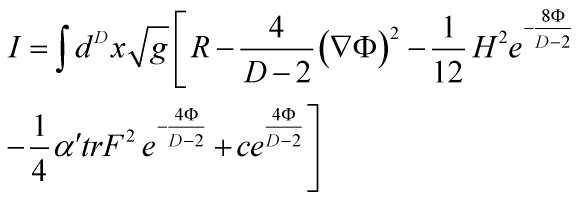
Consider the inverse string tension $\alpha '$ in the Einstein frame with effective string action in D-dimensions:

with

${\left( {\nabla \Phi } \right)^2} = {g^{\mu \nu }}{\nabla _\mu }\Phi {\nabla _\nu }\Phi$

and

$\left\{ {\begin{array}{*{20}{c}}{{H^2} = {H_{\mu \nu \sigma }}{H^{\mu \nu \sigma }}}\\{{{\left( {{F^2}} \right)}_{ab}}{F_{a\mu \nu }}F_b^{\mu \nu }}\end{array}} \right.$

with the heterotic string action being, generically:

and

${H_{\mu \nu \sigma }} = 3{\not \partial _{\left[ {\mu {B_{\nu \sigma }}} \right]}}$

${F_{a\mu \nu }} = {\not \partial _\nu }{A_{a\mu }} - {\not \partial _\mu }{A_{a\nu }} + g{C_{abc}}{A_{b\mu }}{A_{c\nu }}$

Noting that the field ${B_{\mu \nu }}$ is the antisymmetric tensor field, ${A_{a\mu }}$ the background spacetime gauge field. The constant c is the central charge deficit:

$c = - 2\left( {{D_{eff}} - {D_{crit}}} \right)/3\alpha '$

in the heterotic and superstring theories.

The field $\Phi$ is the fundamental scalar field of string theory, the dilaton. Moreover, note that ${\nabla _\mu }$ in the above effective string action in D-dimensions is the covariant spacetime derivative in D-dimensions

and crucial substitutions in the EEA with respect to:

$\left\{ {\begin{array}{*{20}{c}}\Phi \\{{g_{\mu \nu }}}\\{{B_{\mu \nu }}}\\{{A_{a\mu }}}\end{array}} \right.$

gives us:

${\bar \nabla ^2}\Phi + \frac{1}{{12}}{H^2}{e^{ - \frac{{8\Phi }}{{D - 2}}}} + \frac{{\alpha '}}{8}tr{F^2}{e^{ - \frac{{4\Phi }}{{D - 2}}}} + \frac{c}{2}{e^{\frac{{4\Phi }}{{D - 2}}}}$

${R_{\mu \nu }} - \frac{1}{2}{g_{\mu \nu }}R = - {T_{\mu \nu }}$

$\begin{array}{*{20}{l}}{{T_{\mu \nu }} = \frac{8}{{D - 2}}{{\left( {\bar \nabla \Phi } \right)}^2}\left. {{g_{\mu \nu }}} \right] - \frac{1}{2}{e^{ - \frac{{8\Phi }}{{D - 2}}}}\left[ {H_{\mu \nu }^2 - \frac{1}{6}{H^2}{g_{\mu \nu }}} \right]}\\{ - \frac{{\alpha '}}{2}{e^{ - \frac{{4\Phi }}{{D - 2}}}}\left[ {2F_{\mu \nu }^2 - \frac{1}{2}tr{F^2}{g_{\mu \nu }}} \right]}\\{ - c{e^{\frac{{4\Phi }}{{D - 2}}}}{g_{\mu \nu }}}\end{array}$

as well as:

${\nabla _\lambda }\left( {{e^{ - \frac{{8\Phi }}{{D - 2}}}}H_{\mu \nu }^\lambda } \right) = 0$

and:

${\nabla ^\mu }\left( {{F_{a\mu \nu }}{e^{ - \frac{{4\Phi }}{{D - 2}}}}} \right) = g{C_{abc}}A_b^\mu {F_{c\mu \nu }}{e^{ - \frac{{4\Phi }}{{D - 2}}}}$

Now, since I can set $D = 4$ , an exact solution with an homogeneous and isotropic Robertson-Walker metric can be given by

$\begin{array}{l}d{s^2} = - d{t^2} + a{\left( t \right)^2}\left[ {\frac{{d{r^2}}}{{1 - k{r^2}}}} \right. + {r^2}\\\left. {\left( {d{\theta ^2} + {{\sin }^2}\theta d{\varphi ^2}} \right)} \right]\end{array}$

with non-vanishing components:

${R_{ij}} = - \left[ {\frac{{\ddot a}}{a} + \frac{2}{{{a^2}}}\left( {{{\dot a}^2} + k'} \right)} \right]{g_{ij}}$

with:

${R_{00}} = 3\frac{{\ddot a}}{{a'}}$

so that

${R_{\mu \nu }} - \frac{1}{2}{g_{\mu \nu }}R = - {T_{\mu \nu }}$

reduces to:

$3\frac{{\ddot a}}{a} = \left( {T_0^0 - \frac{1}{2}T} \right)$

with:

$\left[ {\frac{{\ddot a}}{a} + \frac{2}{{{a^2}}}\left( {{{\dot a}^2} + } \right)} \right]\delta _j^i = \left( {T_j^i - \frac{1}{2}T\delta _j^i} \right)$

thus allowing us to derive:

$T_j^i \sim \delta _j^i$

given maximal spatial symmetry.

Since in a homogeneous universe, all fields are essentially functions of time, equation:

${\nabla _\lambda }\left( {{e^{ - \frac{{8\Phi }}{{D - 2}}}}H_{\mu \nu }^\lambda } \right) = 0$

has a solution via the ansatz:

${H^{\lambda \mu \nu }} = {\varepsilon ^{\lambda \mu \nu \sigma }}{e^{4\Phi }}{\nabla _\sigma }\rho$

with $\rho = \rho \left( t \right)$ a homogeneous scalar field.

Here is the deep pivot – we can infer that:

${H^2}_\nu ^\mu = {\varepsilon ^{\alpha \beta \mu \sigma }}{\varepsilon _{\alpha \beta \nu \lambda }}{e^{8\Phi }}{\nabla _{\sigma \rho }}{\nabla _{\lambda \rho }}$

can be derived from:

$\left\{ {\begin{array}{*{20}{c}}{{H^2}_j^i = h\left( t \right)\delta _j^i}\\{{H^2}_0^0 = 0}\end{array}} \right.$

with

$h\left( t \right) = - 2{e^{8\Phi }}{\dot \rho ^2}$

Given the fact that $T_j^i \propto \delta _j^i$

then from:

it follows that:

${F^2}_j^i \equiv {F^2}_j^i = f\left( t \right)\delta _j^i$

implying that the field equations:

${\nabla ^\mu }\left( {{F_{a\mu \nu }}{e^{ - \frac{{4\Phi }}{{D - 2}}}}} \right) = g{C_{abc}}A_b^\mu {F_{c\mu \nu }}{e^{ - \frac{{4\Phi }}{{D - 2}}}}$

are solvable obeying the restriction:

${F^2}_j^i \equiv {F^2}_j^i = f\left( t \right)\delta _j^i$

and the tensor ${H^{\lambda \mu \nu }}$ is completely determined by solutions to:

${H^2}_\nu ^\mu = {\varepsilon ^{\alpha \beta \mu \sigma }}{\varepsilon _{\alpha \beta \nu \lambda }}{e^{8\Phi }}{\nabla _{\sigma \rho }}{\nabla _{\lambda \rho }}$

and

$h\left( t \right) = - 2{e^{8\Phi }}{\dot \rho ^2}$

Thus, the right-hand side in equations:

$3\frac{{\ddot a}}{a} = \left( {T_0^0 - \frac{1}{2}T} \right)$

and

$\left[ {\frac{{\ddot a}}{a} + \frac{2}{{{a^2}}}\left( {{{\dot a}^2} + } \right)} \right]\delta _j^i = \left( {T_j^i - \frac{1}{2}T\delta _j^i} \right)$

yield

$\left\{ {\begin{array}{*{20}{c}}{{\nabla _i}\Phi = 0}\\{{F^2}_0^0 = {f_0}}\end{array}} \right.$

hence we have the no-singular cosmology terms:

$\begin{array}{l}T_j^i = \left[ {2{{\left( {\bar \nabla \Phi } \right)}^2} - \frac{1}{4}} \right.{e^{ - 4\Phi }}h - \\\frac{{\alpha '}}{4}{e^{ - 2\Phi }}\left. {\left( {f - {f_0}} \right) - c{e^{2\Phi }}} \right]\delta _j^i\end{array}$

$\left\{ {\begin{array}{*{20}{c}}{{H^2} = 3h}\\{tr{F^2} = 3f + {f_0}}\end{array}} \right.$

and thus, a common property with all quantum gravity theories:

$\begin{array}{l}T_0^0 = 4\left[ {\frac{1}{2}{{\left( {\bar \nabla \Phi } \right)}^2} + {{\dot \Phi }^2}} \right] + \\\frac{1}{4}{e^{ - 4\Phi }}h + \frac{3}{4}\alpha '{e^{ - 2\Phi }}\left( {f - {f_0}} \right) - \\c{e^{2\Phi }}\end{array}$

with

$T \buildrel\textstyle.\over= 4{\left( {\bar \nabla \Phi } \right)^2} - \frac{1}{2}{e^{ - 4\Phi }}h - 4c{e^{2\Phi }}$

Therefore, substituting uniformly with respect to $\dot a$ and $\ddot a$ , the scalar equation:

${\bar \nabla ^2}\Phi + \frac{1}{{12}}{H^2}{e^{ - \frac{{8\Phi }}{{D - 2}}}} + \frac{{\alpha '}}{8}tr{F^2}{e^{ - \frac{{4\Phi }}{{D - 2}}}} + \frac{c}{2}{e^{\frac{{4\Phi }}{{D - 2}}}}$

reduces to:

${\bar \nabla ^2}\Phi + \frac{1}{4}{e^{ - 4\Phi }}h + \frac{{\alpha '}}{8}{e^{ - 2\Phi }}\left( {3f + {f_0}} \right) + \frac{c}{2}{e^{2\Phi }} = 0$

which is a coupled non-linear second order differential equations: let’s look at its behavior at ‘t = 0’.

We have for any field $\phi = 2\Phi$ , the following:

$\left\{ {\begin{array}{*{20}{c}}{a = {a_0}{e^{\phi /2}}}\\{{a^2} = a_0^2 + {t^2}}\end{array}} \right.$

$\phi = - {\rm{In}}\left( {1 + \frac{{{t^2}}}{{a_0^2}}} \right)$

$h = 4\left( {c - \frac{8}{{a_0^2}}} \right){e^{3\phi }} + \frac{{20}}{{a_0^2}}{e^{4\phi }}$

$\alpha 'f = - 2\left( {c - \frac{8}{{a_0^2}}} \right){e^{2\phi }} - \frac{{11}}{{a_0^2}}{e^{3\phi }}$

$\alpha '{f_0} = - 2\left( {3c - \frac{{16}}{{a_0^2}}} \right){e^{2\phi }} - \frac{{15}}{{a_0^2}}{e^{3\phi }}$

Let me sum the philosophical depth now

There is no trace of any ‘big-bang’ initial singularity and without violating the general singularity theorems in classical General Relativity, since the strong energy condition, which is sufficient for the existence of the initial singularity, is avoided by a choice of c within an allowed interval determined by IC and BC.
Also, we have: even though $\phi \to - \infty$ and $\phi \to \infty$ , ${H^2}$ and $tr{F^2}$ vanish in this limit.
The dynamics of the evolution of the theory fleshed in this post, and it is representative, depend only on the existence of the fields F and H. So the Lagrangian density is:

$\tilde L = R - \frac{1}{2}{\left( {\bar \nabla \phi } \right)^2} - V\left( \phi \right)$

with

$V\left( \phi \right) = \frac{1}{{12}}{H^2}{e^{ - 2\phi }} + \frac{{\alpha '}}{4}tr{F^2}{e^{ - \phi }} - c{e^\phi }$

the effective potential. Thus, again, implying a non-singular cosmological scenario!

In turn, to torture the physicists

4-D Effective String-Theory and No-Singularity Cosmology

In this post, I will analyze how non-singular cosmology emerges in heterotic string theory

The field $\Phi$ is the fundamental scalar field of string theory, the dilaton. Moreover, note that ${\nabla _\mu }$ in the above effective string action in D-dimensions is the covariant spacetime derivative in D-dimensions

Now, since I can set $D = 4$ , an exact solution with an homogeneous and isotropic Robertson-Walker metric can be given by

Here is the deep pivot – we can infer that:

Given the fact that $T_j^i \propto \delta _j^i$

Therefore, substituting uniformly with respect to $\dot a$ and $\ddot a$ , the scalar equation:

Let me sum the philosophical depth now

In turn, to torture the physicists

Quantum Geometry, Emergence and Noncommutative Spacetime

Hodge Theory and Gromov-Witten Invariants of Calabi-Yau 3-Folds

About Me

Social Networks

Archives

Login Below

Photo Gallery

In this post, I will analyze how non-singular cosmology emerges in heterotic string theory

The field is the fundamental scalar field of string theory, the dilaton. Moreover, note that in the above effective string action in D-dimensions is the covariant spacetime derivative in D-dimensions

Now, since I can set , an exact solution with an homogeneous and isotropic Robertson-Walker metric can be given by

Here is the deep pivot – we can infer that:

Given the fact that

Therefore, substituting uniformly with respect to and , the scalar equation:

Let me sum the philosophical depth now

In turn, to torture the physicists

Quantum Geometry, Emergence and Noncommutative Spacetime

Hodge Theory and Gromov-Witten Invariants of Calabi-Yau 3-Folds

RELATED

F-theory as the Modular Equivariant 12-D Lift of Type-IIB String Theory

Exceptional Field Theory and M-Theory on Kovalev TCS G2-Manifolds

The Wess–Zumino–Witten–Novikov Model, Taub-NUT Spaces, and M-Theory

About Me

Social Networks

Archives

Login Below

Photo Gallery

The field $\Phi$ is the fundamental scalar field of string theory, the dilaton. Moreover, note that ${\nabla _\mu }$ in the above effective string action in D-dimensions is the covariant spacetime derivative in D-dimensions

Now, since I can set $D = 4$ , an exact solution with an homogeneous and isotropic Robertson-Walker metric can be given by

Given the fact that $T_j^i \propto \delta _j^i$

Therefore, substituting uniformly with respect to $\dot a$ and $\ddot a$ , the scalar equation: